A basic chapter

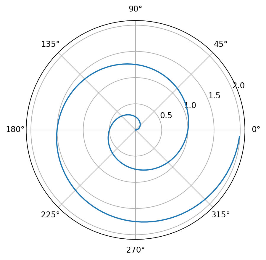
Open the associated notebook:

A beautiful figure

This chunk shows how you can produce a beautiful figure.

Code

import numpy as np
import matplotlib.pyplot as plt

r = np.arange(0, 2, 0.01)
theta = 2 * np.pi * r
fig, ax = plt.subplots(
  subplot_kw = {'projection': 'polar'} 
)
ax.plot(theta, r)
ax.set_rticks([0.5, 1, 1.5, 2])
ax.grid(True)
plt.show()

A beautiful dataframe

This section demonstrates how to create and display a simple pandas DataFrame.

Code

import pandas as pd

data = {
    "Name": ["Alice", "Bob", "Charlie"],
    "Age": [25, 30, 35],
    "City": ["Paris", "Dublin", "Berlin"]
}

df = pd.DataFrame(data)
df

Table 1: Simple pandas DataFrame

	Name	Age	City
0	Alice	25	Paris
1	Bob	30	Dublin
2	Charlie	35	Berlin

A more sophisticated table

This section demonstrates how to create and display a simple pandas DataFrame.

Code

from great_tables import GT, html
from great_tables.data import sza
import polars as pl
from polars import col as c
import polars.selectors as cs

sza_pivot = (
    pl.from_pandas(sza)
    .filter((c.latitude == "20") & (c.tst <= "1200"))
    .select(pl.col("*").exclude("latitude"))
    .drop_nulls()
    .pivot(values="sza", index="month", on="tst", sort_columns=True)
)

(
    GT(sza_pivot, rowname_col="month")
    .data_color(
        domain=[90, 0],
        palette=["rebeccapurple", "white", "orange"],
        na_color="white",
    )
    .tab_header(
        title="Solar Zenith Angles from 05:30 to 12:00",
        subtitle=html("Average monthly values at latitude of 20&deg;N."),
    )
    .sub_missing(missing_text="")
)

	0530	0600	0630	0700	0730	0800	0830	0900	0930	1000	1030	1100	1130	1200
Solar Zenith Angles from 05:30 to 12:00
Average monthly values at latitude of 20°N.
jan				84.9	78.7	72.7	66.1	61.5	56.5	52.1	48.3	45.5	43.6	43.0
feb			88.9	82.5	75.8	69.6	63.3	57.7	52.2	47.4	43.1	40.0	37.8	37.2
mar			85.7	78.8	72.0	65.2	58.6	52.3	46.2	40.5	35.5	31.4	28.6	27.7
apr		88.5	81.5	74.4	67.4	60.3	53.4	46.5	39.7	33.2	26.9	21.3	17.2	15.5
may		85.0	78.2	71.2	64.3	57.2	50.2	43.2	36.1	29.1	26.1	15.2	8.8	5.0
jun	89.2	82.7	76.0	69.3	62.5	55.7	48.8	41.9	35.0	28.1	21.1	14.2	7.3	2.0
jul	88.8	82.3	75.7	69.1	62.3	55.5	48.7	41.8	35.0	28.1	21.2	14.3	7.7	3.1
aug		83.8	77.1	70.2	63.3	56.4	49.4	42.4	35.4	28.3	21.3	14.3	7.3	1.9
sep		87.2	80.2	73.2	66.1	59.1	52.1	45.1	38.1	31.3	24.7	18.6	13.7	11.6
oct			84.1	77.1	70.2	63.3	56.5	49.9	43.5	37.5	32.0	27.4	24.3	23.1
nov			87.8	81.3	74.5	68.3	61.8	56.0	50.2	45.3	40.7	37.4	35.1	34.4
dec				84.3	78.0	71.8	66.1	60.5	55.6	50.9	47.2	44.2	42.4	41.8