Cross-validation based on data structure

Imbalanced data

Goal: Ensure reliable evaluation of model performance when predicting an imbalanced target

Problem: In imbalanced datasets, random folds may not contain enough observations of rare target values, leading to biased or misleading performance estimates

Solution: Stratified K-Fold Cross-Validation, which preserves the distribution of the target variable (QF185001) in each fold

Key message: If you don’t preserve the target distribution, you are no longer evaluating the same problem in each fold

library(rsample)
library(dplyr)

Attaching package: 'dplyr'

The following objects are masked from 'package:stats':

    filter, lag

The following objects are masked from 'package:base':

    intersect, setdiff, setequal, union

library(arrow)

Attaching package: 'arrow'

The following object is masked from 'package:utils':

    timestamp

data_cv0 <-  read_parquet("data/data_synth_cv0.parquet", as_data_frame = TRUE)
set.seed(123)

folds <- vfold_cv(data_cv0, v = 5, strata = QF185001)

split1 <- folds$splits[[1]]

train_data <- analysis(split1)
test_data  <- assessment(split1)

in the case where the variable is continuous like in our case we can use bins

# create the binned varaiable
data_cv0 <- data_cv0 |>
  mutate(QF185001_bin = ntile(QF185001, 5))

# lighter inspection
dplyr::glimpse(data_cv0, width = 60)

Rows: 3,496
Columns: 43
$ ANO          <dbl> 2026, 2026, 2026, 2026, 2026, 2026, 2…
$ DD_CC_FF_COD <chr> "140120", "010312", "050807", "310307…
$ N2_COD_1     <chr> "16", "16", "16", "30", "18", "18", "…
$ ENUT         <chr> "2", "2", "2", "7", "4", "4", "1", "3…
$ L_NUT        <chr> "Centro", "Centro", "Centro", "Madeir…
$ NPS          <dbl> 3, 1, 2, 1, 7, 9, 10, 10, 14, 12, 6, …
$ INQ          <chr> "1", "1", "1", "1", "1", "1", "1", "1…
$ L_EPS        <chr> "1 a 19", "1 a 19", "1 a 19", "1 a 19…
$ VVN          <dbl> 247262, 49222, 49404, 32239, 267866, …
$ EVN          <chr> "2", "1", "1", "1", "3", "3", "4", "3…
$ CAE_BC       <chr> "41200", "43340", "43330", "43390", "…
$ ECAE         <chr> "4120", "4334", "4333", "4339", "4333…
$ ESTRATO      <chr> "41200.B.2", "43340.B.1", "43330.B.1"…
$ AMH          <dbl> 171, 18, 15, 18, 218, 180, 114, 12, 1…
$ UNI          <dbl> 14287, 477, 466, 516, 218, 180, 114, …
$ IMP          <dbl> 0, 0, 0, 0, 0, 0, 0, 0, 0, 0, 0, 0, 0…
$ I187701      <dbl> 0, 0, 0, 0, 0, 0, 0, 0, 0, 0, 0, 0, 0…
$ I20540       <dbl> 0, 0, 0, 0, 0, 0, 0, 0, 0, 0, 0, 0, 0…
$ I20550       <dbl> 0, 0, 0, 0, 0, 0, 0, 0, 0, 0, 0, 0, 0…
$ QF185001     <dbl> 108056, 52986, 54000, 1, 278644, 4704…
$ QF185002     <dbl> 0, 0, 0, 0, 105000, 195000, 0, 0, 0, …
$ QF185003     <dbl> 108056, 52986, 54000, 0, 173644, 1444…
$ QF185004     <dbl> 0, 0, 0, 1, 0, 130952, 0, 421391, 111…
$ QF185101     <dbl> 108056, 52986, 54000, 0, 278644, 2055…
$ QF185501     <dbl> 0, 0, 0, 1, 0, 449891, 1203106, 62659…
$ QF186301     <dbl> 0, 0, 0, 0, 0, 0, 0, 0, 0, 613262, 12…
$ QF186302     <dbl> 0, 0, 0, 0, 0, 0, 0, 0, 0, 613262, 0,…
$ QF186303     <dbl> 0, 0, 0, 0, 0, 0, 0, 0, 0, 0, 0, 0, 0…
$ QF186304     <dbl> 0, 0, 0, 0, 0, 0, 0, 0, 0, 0, 122614,…
$ QF186401     <dbl> 0, 0, 0, 0, 0, 0, 0, 0, 0, 0, 0, 0, 0…
$ QF187001     <dbl> 0, 0, 0, 0, 0, 0, 0, 0, 0, 0, 0, 0, 0…
$ QF187301     <dbl> 0, 0, 0, 0, 0, 0, 0, 0, 0, 582599, 0,…
$ QF187401     <dbl> 0, 0, 0, 0, 0, 0, 0, 0, 0, 30663, 122…
$ QF187701     <dbl> 108056, 52986, 54000, 1, 278644, 4704…
$ QF187702     <dbl> 0, 0, 0, 0, 105000, 195000, 0, 0, 0, …
$ QF187703     <dbl> 108056, 52986, 54000, 0, 173644, 1444…
$ QF187704     <dbl> 0, 0, 0, 1, 0, 130952, 0, 421391, 111…
$ QF20540      <dbl> 0, 0, 0, 0, 0, 0, 0, 0, 0, 0, 0, 0, 0…
$ QF20550      <dbl> 108056, 3255, 1, 1, 10604, 43822, 745…
$ source       <chr> "B", "B", "B", "B", "B", "B", "B", "B…
$ ID           <dbl> 1, 2, 3, 4, 5, 6, 7, 8, 9, 10, 11, 12…
$ unit         <int> 2, 2, 2, 2, 2, 2, 2, 2, 2, 2, 2, 2, 2…
$ QF185001_bin <int> 2, 2, 2, 2, 2, 3, 4, 3, 2, 3, 1, 2, 2…

folds <- vfold_cv(data_cv0, v = 5, strata = QF185001_bin)

data_cv0 %>%
  group_by(QF185001_bin) %>%
  summarise(
    min = min(QF185001, na.rm = TRUE),
    max = max(QF185001, na.rm = TRUE),
    n = n()
  ) %>%
  arrange(QF185001_bin)

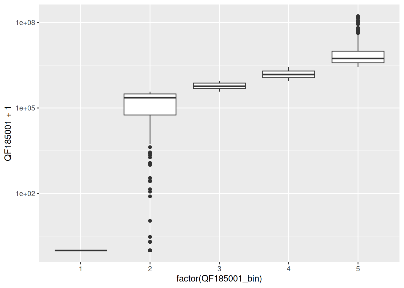
# A tibble: 5 × 4
  QF185001_bin     min       max     n
         <int>   <dbl>     <dbl> <int>
1            1       0         0   700
2            2       0    373699   699
3            3  374281    898483   699
4            4  899268   2751726   699
5            5 2763029 167794350   699

library(ggplot2)

ggplot(data_cv0, aes(x = factor(QF185001_bin), y = QF185001 + 1)) +
  geom_boxplot() +
  scale_y_log10()

Small datasets

Goal: Ensure reliable estimation of model performance when data is limited

Problem: With small datasets, model evaluation has high variance because each split contains very few observations, making results unstable and sensitive to data partitioning

Solution: - Leave-One-Out Cross-Validation (LOOCV): maximizes training data usage - Repeated K-Fold Cross-Validation: reduces variance by averaging across multiple random splits

Key Message: When data is scarce, the main risk is not bias but high variance in evaluation. Use resampling strategies that stabilize results

Leave-One-Out Cross-Validation (LOOCV)

uses all data efficiently but does not scale well, as it requires training one model per observation.

library(rsample)

# keeping only numeric predictors in the example 
data_num <- data_cv0 %>% select(where(is.numeric))

# making a small sample because we will have as many
# folds as observations
data_small <- data_num %>% slice_sample(n = 100) 

folds <- loo_cv(data_small)

length(folds$splits)

[1] 100

s <- folds$splits[[1]]

train <- analysis(s)
test  <- assessment(s)

nrow(train)

[1] 99

nrow(test)

[1] 1

# errs stores the error for each fold
# since each fold has 1 test observation, each value is
# the prediction error for that observation
errs <- sapply(folds$splits, function(s) {
  train <- analysis(s)
  test  <- assessment(s)
  
  # lm is simple example model (linear regression)
  # not required for LOOCV
  # may replace it with any model (tree, random forest, etc.)
  m <- lm(QF185001 ~ ., data = train)
  pred <- predict(m, test)
  
  # mean squared error
  mean((test$QF185001 - pred)^2)
})

# train many models (almost identical)
# each tested on one observation
# then average the errors
mean(errs)

[1] 2.256731e-17

Repeated K-Fold Cross-Validation

Repeated K-Fold reduces variance by averaging over multiple data splits.

library(rsample)

# split data into 5 folds
# repeat the whole process 10 times with different random splits
# Total models trained = 5 × 10 = 50
folds <- vfold_cv(data_cv0, v = 5, repeats = 10)

nrow(folds)

[1] 50

folds$splits[[1]]

<Analysis/Assess/Total>
<2796/700/3496>

s <- folds$splits[[1]]

train <- analysis(s)
test  <- assessment(s)

nrow(train)

[1] 2796

nrow(test)

[1] 700

Train/test separation (~80% / 20%)

library(rpart)

# train many models on different splits
# compute error each time
# and average provide more stable estimate
errs <- sapply(folds$splits, function(s) {
  train <- analysis(s)
  test  <- assessment(s)

  train$ESTRATO <- factor(train$ESTRATO)
test$ESTRATO  <- factor(test$ESTRATO, levels = levels(train$ESTRATO))
  train$DD_CC_FF_COD <- factor(train$DD_CC_FF_COD)
  test$DD_CC_FF_COD  <- factor(test$DD_CC_FF_COD,
                               levels = levels(train$DD_CC_FF_COD))

  m <- rpart(QF185001 ~ ., data = train)
  pred <- predict(m, test)

  mean((test$QF185001 - pred)^2)
})

mean(errs)

[1] 1.046159e+13

data_cv1 <- read_parquet("data/data_synth_cv1.parquet")

dplyr::glimpse(data_cv1)

Rows: 11,075
Columns: 42
$ ANO          <dbl> 2026, 2026, 2026, 2026, 2026, 2026, 2026, 2026, 2026, 202…
$ DD_CC_FF_COD <chr> "140120", "140120", "010312", "010312", "050807", "050807…
$ N2_COD_1     <chr> "16", "16", "16", "16", "16", "16", "30", "30", "30", "18…
$ ENUT         <chr> "2", "2", "2", "2", "2", "2", "7", "7", "7", "4", "4", "4…
$ L_NUT        <chr> "Centro", "Centro", "Centro", "Centro", "Centro", "Centro…
$ NPS          <dbl> 3, 3, 1, 1, 2, 2, 1, 1, 1, 7, 7, 9, 9, 10, 10, 10, 10, 10…
$ INQ          <chr> "1", "1", "1", "1", "1", "1", "1", "1", "1", "1", "1", "1…
$ L_EPS        <chr> "1 a 19", "1 a 19", "1 a 19", "1 a 19", "1 a 19", "1 a 19…
$ VVN          <dbl> 247262, 247262, 49222, 49222, 49404, 49404, 32239, 32239,…
$ EVN          <chr> "2", "2", "1", "1", "1", "1", "1", "1", "1", "3", "3", "3…
$ CAE_BC       <chr> "41200", "41200", "43340", "43340", "43330", "43330", "43…
$ ECAE         <chr> "4120", "4120", "4334", "4334", "4333", "4333", "4339", "…
$ ESTRATO      <chr> "41200.B.2", "41200.B.2", "43340.B.1", "43340.B.1", "4333…
$ AMH          <dbl> 196, 171, 18, 18, 14, 15, 18, 18, 16, 247, 218, 209, 180,…
$ UNI          <dbl> 15223, 14287, 385, 477, 405, 466, 432, 516, 519, 247, 218…
$ IMP          <dbl> 0, 0, 0, 0, 0, 0, 0, 0, 0, 0, 0, 0, 0, 0, 0, 0, 0, 0, 0, …
$ I187701      <dbl> 0, 0, 0, 0, 0, 0, 0, 0, 0, 0, 0, 0, 0, 0, 0, 0, 0, 0, 0, …
$ I20540       <dbl> 0, 0, 0, 0, 0, 0, 0, 0, 0, 0, 0, 0, 0, 0, 0, 0, 0, 0, 0, …
$ I20550       <dbl> 0, 0, 0, 0, 0, 0, 0, 0, 0, 0, 0, 0, 0, 0, 0, 0, 0, 0, 0, …
$ QF185001     <dbl> 106026, 108056, 54611, 52986, 59000, 54000, 1, 1, 1, 2635…
$ QF185002     <dbl> 0, 0, 0, 0, 0, 0, 0, 0, 0, 105000000, 105000, 0, 195000, …
$ QF185003     <dbl> 106026, 108056, 54611, 52986, 59000, 54000, 0, 0, 0, 4555…
$ QF185004     <dbl> 0, 0, 0, 0, 0, 0, 1, 1, 1, 113000540, 0, 0, 130952, 60804…
$ QF185101     <dbl> 106026, 108056, 54611, 52986, 59000, 54000, 1, 0, 1, 1835…
$ QF185501     <dbl> 0, 0, 0, 0, 0, 0, 0, 1, 0, 80019000, 0, 178703, 449891, 6…
$ QF186301     <dbl> 0, 0, 0, 0, 0, 0, 1, 0, 1, 0, 0, 0, 0, 0, 0, 0, 0, 0, 0, …
$ QF186302     <dbl> 0, 0, 0, 0, 0, 0, 0, 0, 0, 0, 0, 0, 0, 0, 0, 0, 0, 0, 0, …
$ QF186303     <dbl> 0, 0, 0, 0, 0, 0, 0, 0, 0, 0, 0, 0, 0, 0, 0, 0, 0, 0, 0, …
$ QF186304     <dbl> 0, 0, 0, 0, 0, 0, 1, 0, 1, 0, 0, 0, 0, 0, 0, 0, 0, 0, 0, …
$ QF186401     <dbl> 0, 0, 0, 0, 0, 0, 0, 0, 0, 0, 0, 0, 0, 0, 0, 0, 0, 0, 0, …
$ QF187001     <dbl> 0, 0, 0, 0, 0, 0, 0, 0, 1, 0, 0, 0, 0, 0, 0, 0, 0, 0, 0, …
$ QF187301     <dbl> 0, 0, 0, 0, 0, 0, 0, 0, 0, 0, 0, 0, 0, 0, 0, 0, 0, 0, 0, …
$ QF187401     <dbl> 0, 0, 0, 0, 0, 0, 1, 0, 0, 0, 0, 0, 0, 0, 0, 0, 0, 0, 0, …
$ QF187701     <dbl> 106026, 108056, 54611, 52986, 59000, 54000, 2, 1, 2, 2635…
$ QF187702     <dbl> 0, 0, 0, 0, 0, 0, 0, 0, 0, 105000000, 105000, 0, 195000, …
$ QF187703     <dbl> 106026, 108056, 54611, 52986, 59000, 54000, 0, 0, 0, 4555…
$ QF187704     <dbl> 0, 0, 0, 0, 0, 0, 2, 1, 2, 113000540, 0, 0, 130952, 60804…
$ QF20540      <dbl> 0, 0, 0, 0, 0, 0, 0, 0, 1, 0, 0, 0, 0, 0, 0, 371853, 0, 0…
$ QF20550      <dbl> 5417, 108056, 3017, 3255, 1, 1, 1, 1, 1, 263554540, 10604…
$ source       <chr> "A", "B", "A", "B", "A", "B", "A", "B", "C", "A", "B", "A…
$ ID           <dbl> 1, 1, 2, 2, 3, 3, 4, 4, 4, 5, 5, 6, 6, 7, 7, 7, 8, 8, 8, …
$ unit         <int> 1, 2, 1, 2, 1, 2, 1, 2, 3, 1, 2, 1, 2, 1, 2, 3, 1, 2, 3, …

Grouped / clustered data

Goal: Ensure that model evaluation does not leak information across related observations

Problem: Observations from the same entity (e.g. entreprise) are not independent If split randomly, the same entreprise can appear in both train and test, i.e. data leakage

Solution: Use Group K-Fold Cross-Validation, ensuring that all observations from the same group stay in the same fold

Key Message: If groups are split across folds, the model is evaluated on data it has effectively already seen

Examples: - multiple rows per user - entreprises, households, devices, patients

Group K-Fold Cross-Validation

Same entreprise appears multiple times, requires clustered data - ID - entreprise (group) - unit - establishment (multiple per entreprise)

library(rsample)

folds <- group_vfold_cv(data_cv1, group = ID, v = 5)

s <- folds$splits[[1]]

train <- analysis(s)
test  <- assessment(s)

head(unique(train$ID), 10)

 [1]  2  3  4  5  6  7 10 12 13 14

head(unique(test$ID), 10)

 [1]  1  8  9 11 19 21 25 31 33 36

# check no overlap in groups
intersect(unique(train$ID), unique(test$ID))

numeric(0)

For contrast we will compare with Random CV where we will see overlap

folds_random <- vfold_cv(data_cv1, v = 5)

s <- folds_random$splits[[1]]

train_r <- analysis(s)
test_r  <- assessment(s)

intersect(unique(train_r$ID), unique(test_r$ID))[1:50]

 [1]   1   4   5   7   8   9  10  11  15  18  20  23  25  26  28  30  31  40  41
[20]  42  43  45  51  58  65  69  70  77  82  84  86  87  89  95  96  97  98  99
[39] 101 103 107 108 111 113 114 115 118 125 126 128

Hierarchical / multi-level data

Examples: establishments within entreprises, individuals within households, students within schools Solutions: Nested grouping strategies combine: Group CV + Stratification

Problem: rsample does not natively support group + strata simultaneously How: 1 - Stratify at group level 2 - Split at group level 3 - Apply at observation level

library(dplyr)
data_synth<-data_cv1
df_grouped <- data_synth %>%
  group_by(ID) %>%
  summarise(
    QF185001_mean = mean(QF185001, na.rm = TRUE)
  ) %>%
  mutate(strata = ntile(QF185001_mean, 5))

dplyr::glimpse(df_grouped, width = 60)

Rows: 5,076
Columns: 3
$ ID            <dbl> 1, 2, 3, 4, 5, 6, 7, 8, 9, 10, 11, 1…
$ QF185001_mean <dbl> 107041.0, 53798.5, 56500.0, 1.0, 131…
$ strata        <int> 2, 2, 2, 2, 5, 3, 4, 3, 3, 3, 1, 2, …

library(rsample)

folds_groups <- vfold_cv(df_grouped, v = 5, strata = strata)

folds <- lapply(folds_groups$splits, function(s) {
  
  train_ids <- analysis(s)$ID
  test_ids  <- assessment(s)$ID
  
  list(
    train = data_synth %>% filter(ID %in% train_ids),
    test  = data_synth %>% filter(ID %in% test_ids)
  )
})

f <- folds[[1]]

train <- f$train
test  <- f$test

# check IDs don't overlap
intersect(unique(train$ID), unique(test$ID))

numeric(0)

# Show first IDs
head(unique(train$ID), 10)

 [1]  2  4  5  6  7 10 11 12 14 15

head(unique(test$ID), 10)

 [1]  1  3  8  9 13 34 36 37 44 46

# show units inside one enterprise
train %>%
  filter(ID == train$ID[1]) %>%
  select(ID, unit) %>%
  distinct()

# A tibble: 2 × 2
     ID  unit
  <dbl> <int>
1     2     1
2     2     2

# compare structures
train %>%
  count(ID) %>%
  head()

# A tibble: 6 × 2
     ID     n
  <dbl> <int>
1     2     2
2     4     3
3     5     2
4     6     2
5     7     3
6    10     3

test %>%
  count(ID) %>%
  head()

# A tibble: 6 × 2
     ID     n
  <dbl> <int>
1     1     2
2     3     2
3     8     3
4     9     2
5    13     2
6    34     2

# number of units per entreprise
train %>%
  group_by(ID) %>%
  summarise(n_units = n()) %>%
  summary()

       ID          n_units     
 Min.   :   2   Min.   :1.000  
 1st Qu.:1274   1st Qu.:1.000  
 Median :2548   Median :2.000  
 Mean   :2540   Mean   :2.174  
 3rd Qu.:3792   3rd Qu.:3.000  
 Max.   :5076   Max.   :3.000  

errs <- sapply(folds, function(f) {
  
  train <- f$train
  test  <- f$test
  
  pred <- mean(train$QF185001)
  
  mean((test$QF185001 - pred)^2)
})

mean(errs)

[1] 1.085161e+14

data_cv2 <- read_parquet("data/data_synth_cv2.parquet")

dplyr::glimpse(data_cv2, width = 60)

Rows: 11,075
Columns: 42
$ ANO          <dbl> 2026, 2025, 2026, 2025, 2026, 2025, 2…
$ DD_CC_FF_COD <chr> "140120", "140120", "010312", "010312…
$ N2_COD_1     <chr> "16", "16", "16", "16", "16", "16", "…
$ ENUT         <chr> "2", "2", "2", "2", "2", "2", "7", "7…
$ L_NUT        <chr> "Centro", "Centro", "Centro", "Centro…
$ NPS          <dbl> 3, 3, 1, 1, 2, 2, 1, 1, 1, 7, 7, 9, 9…
$ INQ          <chr> "1", "1", "1", "1", "1", "1", "1", "1…
$ L_EPS        <chr> "1 a 19", "1 a 19", "1 a 19", "1 a 19…
$ VVN          <dbl> 247262, 247262, 49222, 49222, 49404, …
$ EVN          <chr> "2", "2", "1", "1", "1", "1", "1", "1…
$ CAE_BC       <chr> "41200", "41200", "43340", "43340", "…
$ ECAE         <chr> "4120", "4120", "4334", "4334", "4333…
$ ESTRATO      <chr> "41200.B.2", "41200.B.2", "43340.B.1"…
$ AMH          <dbl> 196, 171, 18, 18, 14, 15, 18, 18, 16,…
$ UNI          <dbl> 15223, 14287, 385, 477, 405, 466, 432…
$ IMP          <dbl> 0, 0, 0, 0, 0, 0, 0, 0, 0, 0, 0, 0, 0…
$ I187701      <dbl> 0, 0, 0, 0, 0, 0, 0, 0, 0, 0, 0, 0, 0…
$ I20540       <dbl> 0, 0, 0, 0, 0, 0, 0, 0, 0, 0, 0, 0, 0…
$ I20550       <dbl> 0, 0, 0, 0, 0, 0, 0, 0, 0, 0, 0, 0, 0…
$ QF185001     <dbl> 106026, 108056, 54611, 52986, 59000, …
$ QF185002     <dbl> 0.00e+00, 0.00e+00, 0.00e+00, 0.00e+0…
$ QF185003     <dbl> 106026, 108056, 54611, 52986, 59000, …
$ QF185004     <dbl> 0, 0, 0, 0, 0, 0, 1, 1, 1, 113000540,…
$ QF185101     <dbl> 106026, 108056, 54611, 52986, 59000, …
$ QF185501     <dbl> 0, 0, 0, 0, 0, 0, 0, 1, 0, 80019000, …
$ QF186301     <dbl> 0, 0, 0, 0, 0, 0, 1, 0, 1, 0, 0, 0, 0…
$ QF186302     <dbl> 0, 0, 0, 0, 0, 0, 0, 0, 0, 0, 0, 0, 0…
$ QF186303     <dbl> 0, 0, 0, 0, 0, 0, 0, 0, 0, 0, 0, 0, 0…
$ QF186304     <dbl> 0, 0, 0, 0, 0, 0, 1, 0, 1, 0, 0, 0, 0…
$ QF186401     <dbl> 0, 0, 0, 0, 0, 0, 0, 0, 0, 0, 0, 0, 0…
$ QF187001     <dbl> 0, 0, 0, 0, 0, 0, 0, 0, 1, 0, 0, 0, 0…
$ QF187301     <dbl> 0, 0, 0, 0, 0, 0, 0, 0, 0, 0, 0, 0, 0…
$ QF187401     <dbl> 0, 0, 0, 0, 0, 0, 1, 0, 0, 0, 0, 0, 0…
$ QF187701     <dbl> 106026, 108056, 54611, 52986, 59000, …
$ QF187702     <dbl> 0.00e+00, 0.00e+00, 0.00e+00, 0.00e+0…
$ QF187703     <dbl> 106026, 108056, 54611, 52986, 59000, …
$ QF187704     <dbl> 0, 0, 0, 0, 0, 0, 2, 1, 2, 113000540,…
$ QF20540      <dbl> 0, 0, 0, 0, 0, 0, 0, 0, 1, 0, 0, 0, 0…
$ QF20550      <dbl> 5417, 108056, 3017, 3255, 1, 1, 1, 1,…
$ source       <chr> "A", "B", "A", "B", "A", "B", "A", "B…
$ ID           <dbl> 1, 1, 2, 2, 3, 3, 4, 4, 4, 5, 5, 6, 6…
$ unit         <int> 1, 2, 1, 2, 1, 2, 1, 2, 3, 1, 2, 1, 2…

Time series / temporal data

Goal: Ensure realistic evaluation when predicting future values from past data

Problem: training data may include future observations which leads to data leakage and results in performance being overly optimistic

Solutions: - TimeSeriesSplit - train on past, test on future, - Rolling window - fixed-size moving training window, - Expanding window - training set grows over time

Key Message: If you train on the future to predict the past, you are no longer solving a real-world problem.

Example: the dataset has the same enterprise in several years

TimeSeriesSplit

This is a manual implementation of TimeSeriesSplit using an expanding window.

library(dplyr)

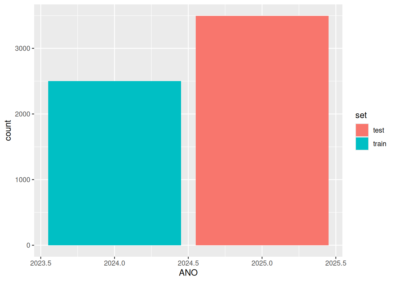
data_ts <- data_cv2 %>%
  arrange(ANO)

data_ts %>% count(ANO)

# A tibble: 3 × 2
    ANO     n
  <dbl> <int>
1  2024  2503
2  2025  3496
3  2026  5076

years <- sort(unique(data_ts$ANO))

# each fold trains on past years and tests on the next year
folds <- lapply(2:length(years), function(i) {
  
  train_years <- years[1:(i-1)]
  test_year   <- years[i]
  
  list(
    train = data_ts %>% filter(ANO %in% train_years),
    test  = data_ts %>% filter(ANO == test_year)
  )
})

f <- folds[[1]]

train <- f$train
test  <- f$test

range(train$ANO)

[1] 2024 2024

range(test$ANO)

[1] 2025 2025

# check no leakage
max(train$ANO) < min(test$ANO)

[1] TRUE

library(ggplot2)

plot_data <- bind_rows(
  train %>% mutate(set = "train"),
  test  %>% mutate(set = "test")
)

ggplot(plot_data, aes(x = ANO, fill = set)) +
  geom_bar(position = "dodge")

errs <- sapply(folds, function(f) {
  
  train <- f$train
  test  <- f$test
  
  pred <- mean(train$QF185001)
  
  mean((test$QF185001 - pred)^2)
})

mean(errs)

[1] 1.076309e+14

Rolling Window

Evaluate models using recent past only, mimicking scenarios where older data becomes less relevant

library(dplyr)

data_ts <- data_cv2 %>%
  arrange(ANO)

years <- sort(unique(data_ts$ANO))
window <- 2  # number of past years to use

folds_roll <- lapply((window+1):length(years), function(i) {
  
  train_years <- years[(i-window):(i-1)]
  test_year   <- years[i]
  
  list(
    train = data_ts %>% filter(ANO %in% train_years),
    test  = data_ts %>% filter(ANO == test_year)
  )
})

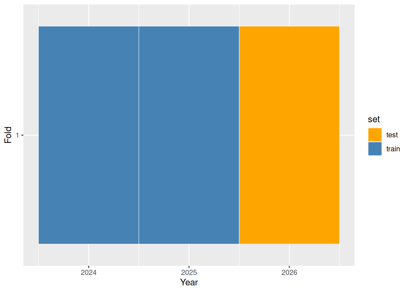
library(ggplot2)

plot_folds <- lapply(seq_along(folds_roll), function(i) {
  
  f <- folds_roll[[i]]
  
  bind_rows(
    f$train %>% distinct(ANO) %>% mutate(set = "train", fold = i),
    f$test  %>% distinct(ANO) %>% mutate(set = "test",  fold = i)
  )
}) %>% bind_rows()

ggplot(plot_folds, aes(x = ANO, y = factor(fold), fill = set)) +
  geom_tile(color = "white") +
  scale_fill_manual(values = c(train = "steelblue", test = "orange")) +
  labs(y = "Fold", x = "Year")

f <- folds_roll[[1]]

range(f$train$ANO)

[1] 2024 2025

range(f$test$ANO)

[1] 2026 2026

max(f$train$ANO) < min(f$test$ANO)

[1] TRUE

errs <- sapply(folds_roll, function(f) {
  
  train <- f$train
  test  <- f$test
  
  pred <- mean(train$QF185001)
  
  mean((test$QF185001 - pred)^2)
})

mean(errs)

[1] 1.367613e+14

Expanding windows

Assume that all past data remains relevant

library(dplyr)

data_ts <- data_cv2 %>%
  arrange(ANO)

years <- sort(unique(data_ts$ANO))

folds_exp <- lapply(2:length(years), function(i) {
  
  train_years <- years[1:(i-1)]
  test_year   <- years[i]
  
  list(
    train = data_ts %>% filter(ANO %in% train_years),
    test  = data_ts %>% filter(ANO == test_year)
  )
})

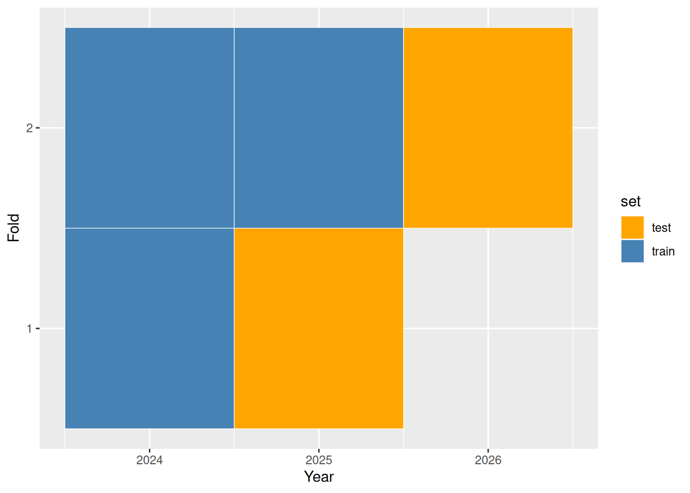
library(ggplot2)

plot_folds_exp <- lapply(seq_along(folds_exp), function(i) {
  
  f <- folds_exp[[i]]
  
  bind_rows(
    f$train %>% distinct(ANO) %>% mutate(set = "train", fold = i),
    f$test  %>% distinct(ANO) %>% mutate(set = "test",  fold = i)
  )
}) %>% bind_rows()

ggplot(plot_folds_exp, aes(x = ANO, y = factor(fold), fill = set)) +
  geom_tile(color = "white") +
  scale_fill_manual(values = c(train = "steelblue", test = "orange")) +
  labs(y = "Fold", x = "Year")

Group + Time - You may need to use a combination of methods

Goal: Ensure evaluation is realistic when data has multiple entities (groups) observed over time

Problem - If we don’t control both we may have: - Group leakage - same enterprise in train and test - Time leakage - future data present in train and the model may learn patterns that are impossible in the real world

Solution: Combine Split by time (respect time order) Grouping by entity (keeping the enterprises in group)

Key Message: When data has both group and time structure, you must respect both. Otherwise, leakage is unavoidable.

data_ts <- data_cv2 %>%
  arrange(ANO)

Each enterprise appears in several years but never shows in the future within the train

years <- sort(unique(data_ts$ANO))

# time first, groups preserved automatically
folds_gt <- lapply(2:length(years), function(i) {
  
  train_years <- years[1:(i-1)]
  test_year   <- years[i]
  
  list(
    train = data_ts %>% filter(ANO %in% train_years),
    test  = data_ts %>% filter(ANO == test_year)
  )
})

library(ggplot2)
library(dplyr)

plot_folds_gt <- lapply(seq_along(folds_gt), function(i) {
  
  f <- folds_gt[[i]]
  
  bind_rows(
    f$train %>% mutate(set = "train", fold = i),
    f$test  %>% mutate(set = "test",  fold = i)
  ) %>%
    distinct(ID, ANO, set, fold)
}) %>% bind_rows()

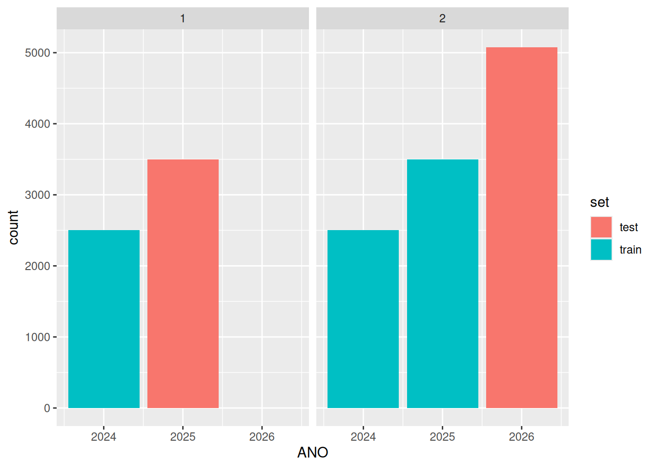
ggplot(plot_folds_gt, aes(x = ANO, fill = set)) +
  geom_bar(position = "dodge") +
  facet_wrap(~ fold)

f <- folds_gt[[1]]

# as expected the same enterprise is present in train and test
intersect(unique(f$train$ID), unique(f$test$ID))[1:50]

 [1]   4   7   8  10  11  12  14  15  18  20  23  26  28  29  43  44  49  51  54
[20]  65  68  69  70  72  78  81  82  84  87  88  92  93  96  97  99 101 102 103
[39] 105 107 109 110 112 113 114 115 117 118 121 122

# but never in the same year
max(f$train$ANO) < min(f$test$ANO)

[1] TRUE

Model selection vs performance estimation

This model is illustative and is not supposed to be executed

Goal: Distinguish between choosing the best model and estimating its real-world performance

Problem: If you use the same data for both you optimize and evaluate on the same information which leads to optimistic bias and performance looks better than it really is

Solution: Separate the processes - Inner loop Model selection (tuning, comparing models) - Outer loop - Performance estimation (unbiased evaluation) This is typically done with nested cross-validation

Key Message: If you evaluate a model on the same data used to select it, you are measuring optimism, not performance.

library(rsample)

folds <- group_vfold_cv(data_cv1, group = ID, v = 5)

outer_folds <- folds  

Nested Cross-Validation prevents overfitting during hyperparameter tuning

library(rsample)
library(dplyr)

errs <- sapply(outer_folds, function(f) {
  
  train_outer <- f$train
  test_outer  <- f$test
  
  # --- INNER CV (model selection) ---
  inner_folds <- vfold_cv(train_outer, v = 5)
  
  model_errors <- sapply(inner_folds$splits, function(s) {
    
    train <- analysis(s)
    test  <- assessment(s)
    
    # Model 1: mean
    pred1 <- mean(train$QF185001)
    err1 <- mean((test$QF185001 - pred1)^2)
    
    # Model 2: linear model
    m <- lm(QF185001 ~ ., data = train)
    pred2 <- predict(m, test)
    err2 <- mean((test$QF185001 - pred2)^2)
    
    c(err1, err2)
  })
  
  # average inner CV error per model
  avg_errs <- rowMeans(model_errors)
  
  # select best model
  best_model <- which.min(avg_errs)
  
  # --- RETRAIN on full outer train ---
  if (best_model == 1) {
    pred <- mean(train_outer$QF185001)
    test_err <- mean((test_outer$QF185001 - pred)^2)
  } else {
    m <- lm(QF185001 ~ ., data = train_outer)
    pred <- predict(m, test_outer)
    test_err <- mean((test_outer$QF185001 - pred)^2)
  }
  
  test_err
})

mean(errs)

This looks like standard CV, but it is incorrect for this dataset.

Goal: Distinguish between choosing the best model and estimating its real-world performan

Spatial data

Examples: geolocation, environmental data

Problem: spatial autocorrelation

Solutions: Spatial blocking, Leave-location-out (nearby points ≠ independent)