NACE recodification with RAG: a reproducible pipeline on SSPCloud

Open this tutorial as an interactive notebook:

Tip

Running the cells interactively? A Python virtual environment has already been created for you (WP10-Cluster5-nace-revision/.venv/bin/python). Click the kernel selector in the top-right corner of the notebook and pick that environment before running any cell.

1 Goal of this tutorial

This tutorial is inspired by subject 2 of the 2026 funathon. See its dedicated website: https://aiml4os.github.io/funathon-project2/.

This tutorial shows a Retrieval-Augmented Generation (RAG) pipeline for an automatic-coding use case: recoding free-text descriptions of economic activities into the new NACE 2.1 nomenclature. The whole pipeline runs end-to-end on the SSPCloud (Insee’s open-source data-science platform): a Qdrant vector database for retrieval, the llm.lab gateway for embeddings and generation, and S3 / MinIO for the data. The same recipe applies to any statistical nomenclature or controlled vocabulary, and to any environment that exposes an OpenAI-compatible LLM endpoint and a Qdrant instance.

Compared to the more pedagogical funathon-project2 tutorial, this notebook is direct: every step of the RAG pipeline is shown with its working code, without question/answer scaffolding.

1.1 Why RAG for recodification?

When a classification is revised (NACE 2.0 → NACE 2.1, COICOP, ISCO, …), the legacy training labels are in the wrong space and a new manual-annotation campaign large enough to retrain a classifier from scratch typically does not yet exist. Asking an LLM to recode from memory is fragile: it confuses adjacent codes, hallucinates codes that do not exist, or mixes up versions of the classification.

RAG splits the task in two:

Retrieve: find the NACE 2.1 codes whose definitions are semantically closest to the activity label, using a vector database.
Generate: ask an LLM to pick the best code from the retrieved shortlist, not from memory.

The knowledge about the nomenclature lives in the vector store, not in the LLM weights. Updating to the next revision means re-indexing, not retraining.

1.2 What this notebook covers

Stage 1: build the vector database once (§3).

Raw NACE 2.1 -> NaceDocument -> Embedding -> Qdrant collection

Stage 2: query the vector database for each activity label, then score the pipeline (§4 and §5).

Activity label -> Embed -> Retrieve top-k (from Qdrant collection)
                         -> Build prompt -> LLM JSON output -> Evaluation metrics

The activity-label evaluation dataset is reused as-is from funathon-project2 (English labels generated by an agentic AI system at low temperature).

2 Technical requirements

2.1 Services

Service	Role
Qdrant	Vector database storing NACE 2.1 embeddings
llm.lab	LLM provider (embedding model + generative model)

2.2 Credentials

Create a .env file with the following variables:

QDRANT_URL=https://YOURNAMESPACE-qdrant.user.lab.sspcloud.fr/
QDRANT_API_KEY=xxxxxxxxxxxxxxxxxxxx
QDRANT_API_PORT=443
LLMLAB_API_KEY=xxxxxxxxxxxxxxxxxxxx
LLMLAB_URL=https://llm.lab.sspcloud.fr/api

Warning

Never commit your .env file. It is already listed in .gitignore. Leaking API keys can expose your services to unauthorised use.

Note

Where to put .env. Put .env at the root of this repository — whether you cloned it yourself, or launched it through the “Open this tutorial as an interactive notebook” button above (which downloads the notebook straight into the cloned repository folder).

2.2.1 Getting your llm.lab API key

Go to the llm.lab interface and sign in with your SSPCloud account.
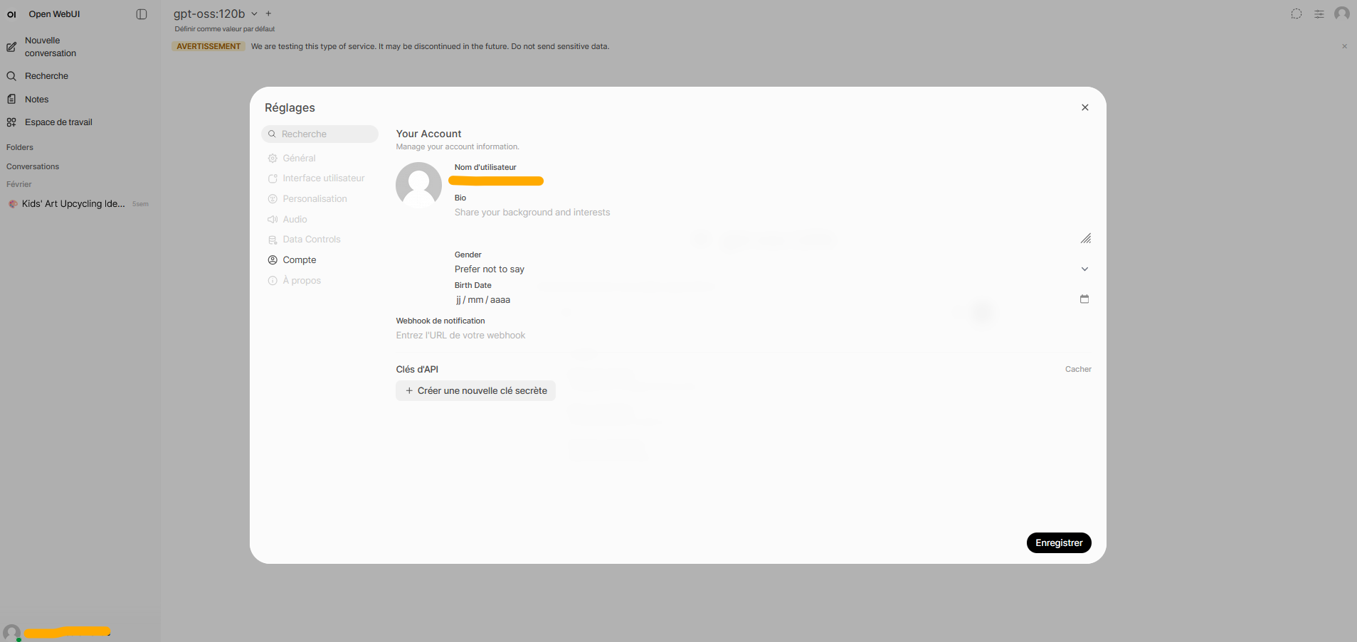
Open Settings (top right) → Account → API Keys.
Generate a new key and copy it into LLMLAB_API_KEY.

2.2.2 Getting your Qdrant credentials

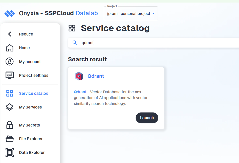
Launch a Qdrant service in your personal SSPCloud namespace.

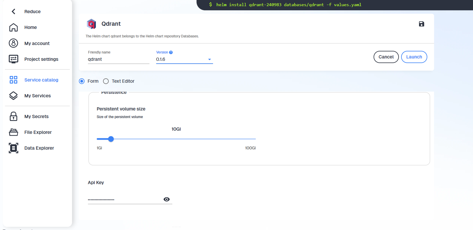
Copy the generated token and save it as QDRANT_API_KEY. The URL follows the pattern https://YOURNAMESPACE-qdrant.user.lab.sspcloud.fr/.

2.3 Loading credentials in Python

from dotenv import load_dotenv
load_dotenv()

To verify a variable was loaded:

import os
try:
    QDRANT_URL = os.environ["QDRANT_URL"]
    print("QDRANT_URL loaded successfully")
except KeyError:
    raise ValueError("QDRANT_URL is not set; check your .env file")

3 Build the vector database

3.1 Connections

import os
from dotenv import load_dotenv
from openai import OpenAI
from qdrant_client import QdrantClient

load_dotenv()

client_llmlab = OpenAI(
    base_url=os.environ["LLMLAB_URL"],
    api_key=os.environ["LLMLAB_API_KEY"],
)

client_qdrant = QdrantClient(
    url=os.environ["QDRANT_URL"],
    api_key=os.environ["QDRANT_API_KEY"],
    port=os.environ["QDRANT_API_PORT"],
)

print("Available llm.lab models:")
for model in client_llmlab.models.list().data:
    print(f"  - {model.id}")

Available llm.lab models:

  - gemma4-26b-moe
  - qwen3-6-35b-moe
  - qwen3-vl
  - qwen3-embedding-8b

3.2 Load the NACE 2.1 nomenclature

The official NACE 2.1 structure (codes, headings, hierarchy, Includes / Excludes notes) is pulled from S3 / MinIO.

import duckdb

PATH_NACE = (
    "https://minio.lab.sspcloud.fr/projet-formation/diffusion/funathon/2026"
    "/project2/NACE_Rev2.1_Structure_Explanatory_Notes_EN.tsv"
)

con = duckdb.connect(database=":memory:")
con.execute("INSTALL httpfs; LOAD httpfs;")
nace = con.execute(f"SELECT * FROM read_csv('{PATH_NACE}')").fetch_arrow_table().to_pylist()

print(f"Loaded {len(nace)} NACE 2.1 entries")
print({k: nace[22][k] for k in ("CODE", "HEADING", "LEVEL")})

Loaded 1047 NACE 2.1 entries
{'CODE': '01.4', 'HEADING': 'Animal production', 'LEVEL': 3}

3.3 `NaceDocument`: clean text + embedding + Qdrant point

One class carries every step from raw row to Qdrant point. The text field is what the embedding model sees; the payload is what retrieval returns.

from dataclasses import dataclass, field
from typing import Optional, List
from uuid import uuid5, NAMESPACE_DNS

from qdrant_client.models import PointStruct

NACE_NAMESPACE = uuid5(NAMESPACE_DNS, "nace-rev2.1")


def _clean(value) -> Optional[str]:
    if value is None:
        return None
    cleaned = " ".join(str(value).replace("\n", " ").split())
    return cleaned or None


@dataclass
class NaceDocument:
    code: str
    heading: str
    level: int
    parent_code: Optional[str] = None
    includes: Optional[str] = None
    includes_also: Optional[str] = None
    excludes: Optional[str] = None

    text: str = field(init=False)
    vector: Optional[List[float]] = field(default=None, init=False)

    @classmethod
    def from_raw(cls, raw: dict, *, with_includes_also: bool = True, with_excludes: bool = True) -> "NaceDocument":
        for key in ("CODE", "HEADING", "LEVEL"):
            if not raw.get(key):
                raise ValueError(f"Missing required field: {key}")
        level = int(raw["LEVEL"])
        if not (1 <= level <= 4):
            raise ValueError(f"Invalid level: {level}")

        obj = cls(
            code=str(raw["CODE"]).strip(),
            heading=_clean(raw["HEADING"]),
            level=level,
            parent_code=_clean(raw.get("PARENT_CODE")),
            includes=_clean(raw.get("Includes")),
            includes_also=_clean(raw.get("IncludesAlso")),
            excludes=_clean(raw.get("Excludes")),
        )
        obj.text = obj.to_embedding_text(with_includes_also=with_includes_also, with_excludes=with_excludes)
        return obj

    def to_embedding_text(self, *, with_includes_also: bool = True, with_excludes: bool = True) -> str:
        parts = [f"# Code: {self.code}", f"# Title: {self.heading}"]
        if self.includes:
            parts += ["", "## Includes:", self.includes.strip()]
        if with_includes_also and self.includes_also:
            parts += ["", "## Also includes:", self.includes_also.strip()]
        if with_excludes and self.excludes:
            parts += ["", "## Excludes:", self.excludes.strip()]
        return "\n".join(parts).replace("\\n", "\n").strip()

    def get_embedding(self, client_llmlab, emb_model: str) -> List[float]:
        response = client_llmlab.embeddings.create(model=emb_model, input=self.text)
        self.vector = response.data[0].embedding
        return self.vector

    def to_qdrant_point(self) -> PointStruct:
        if self.vector is None:
            raise ValueError(f"Vector is missing for code {self.code}")
        return PointStruct(
            id=str(uuid5(NACE_NAMESPACE, self.code)),
            vector=self.vector,
            payload={
                "code": self.code,
                "level": self.level,
                "parent_code": self.parent_code,
                "text": self.text,
            },
        )


nace_documents = [NaceDocument.from_raw(raw) for raw in nace]
print(f"Built {len(nace_documents)} NaceDocument objects")
print("\nExample text (used as embedding input):\n")
print(nace_documents[50].text)

Built 1047 NaceDocument objects

Example text (used as embedding input):

# Code: 03.11
# Title: Marine fishing

## Includes:
This class includes:
- fishing on a commercial basis in ocean and coastal waters
- taking of marine crustaceans and molluscs
- whaling
- taking of marine aquatic animals (e.g. turtles, sea squirts, tunicates, sea urchins)

## Also includes:
This class also includes:
- gathering of other marine organisms and materials (e.g. natural pearls, sponges, coral, seaweed, algae)

## Excludes:
This class excludes:
- capturing of marine mammals apart from whales (e.g. seals, walruses), see 01.70
- processing of whales on factory ships, see 10.11
- processing of fish, crustaceans and molluscs on factory ships or in factories ashore, see 10.20
- rental of pleasure boats with crew for sea and coastal water transport (e.g. for fishing trips), see 50.10
- fishing inspection, protection and patrol services, see 84.24
- fishing practiced for sport or recreation and related services, see 93.19
- operation of sport fishing preserves, see 93.19

3.4 Create the Qdrant collection

from qdrant_client.models import Distance, VectorParams

EMB_MODEL = "qwen3-embedding-8b"
EMB_DIM = 4096
COLLECTION_NAME = "nace-collection"

if client_qdrant.collection_exists(collection_name=COLLECTION_NAME):
    client_qdrant.delete_collection(collection_name=COLLECTION_NAME)

client_qdrant.create_collection(
    collection_name=COLLECTION_NAME,
    vectors_config=VectorParams(size=EMB_DIM, distance=Distance.COSINE),
)
print(f"Collection '{COLLECTION_NAME}' created ({EMB_DIM}-dim, cosine).")

3.5 Embed every entry and upload to Qdrant

upsert is idempotent on the deterministic UUID, so re-running this cell after a failure does not create duplicates.

from more_itertools import chunked
from tqdm import tqdm

BATCH_SIZE = 16

for doc in tqdm(nace_documents, desc="Embedding", unit="doc"):
    doc.get_embedding(client_llmlab, EMB_MODEL)

nace_points = [doc.to_qdrant_point() for doc in nace_documents]

for batch in tqdm(list(chunked(nace_points, BATCH_SIZE)), desc="Uploading", unit="batch"):
    client_qdrant.upsert(collection_name=COLLECTION_NAME, points=batch)

print(f"Collection size: {client_qdrant.count(collection_name=COLLECTION_NAME)}")

Note

For ~1k documents this sequential loop is fine; for production-scale corpora, batch the embedding requests, run them concurrently with bounded concurrency, save progressively, and rely on the deterministic UUIDs for retry safety.

4 Run the RAG pipeline

4.1 Global parameters and prompt

SAMPLE_SIZE = 100

EMB_MODEL_NAME = "qwen3-embedding-8b"
GEN_MODEL_NAME = "gemma4-26b-moe"

RETRIEVER_LIMIT = 5
TEMPERATURE = 0.1

A recodification prompt has three jobs: pin the task to NACE 2.1, constrain the output to the retrieved candidates, and force a JSON shape so parsing is deterministic.

SYSTEM_PROMPT = """\
You are an expert classifier for the NACE 2.1 nomenclature (Statistical Classification of Economic Activities in the European Community, revision 2.1).

You are given a free-text description of an economic activity that needs to be recoded into NACE 2.1, together with a shortlist of candidate NACE 2.1 codes retrieved by a semantic search engine. Your job is to pick the single most appropriate code from the candidates, or to declare the activity not codable if the description is too ambiguous.

Always reply with a valid JSON object matching the requested schema. No explanations, no extra text.
"""

USER_PROMPT_TEMPLATE = """\
## Activity to recode in NACE 2.1
{activity}

## Candidate NACE 2.1 codes and their explanatory notes
{proposed_nace_descriptions}

## Rules
- Pick exactly one code from this list: [{proposed_nace_codes}]. Do not invent codes outside the list.
- If several activities are mentioned, only consider the first one.
- If the description is too vague to decide, return `nace_code: null` and `codable: false`.

## Output (valid JSON only)
{{
  "nace_code": "<one code from the candidate list, or null>",
  "codable": <true | false>,
  "confidence": <float between 0.0 and 1.0>
}}
"""

4.2 Pipeline function

import json


def run_rag_pipeline(activity: str) -> dict:
    # [1] Embed
    embedding = client_llmlab.embeddings.create(
        model=EMB_MODEL_NAME, input=activity
    ).data[0].embedding

    # [2] Retrieve
    points = client_qdrant.query_points(
        collection_name=COLLECTION_NAME, query=embedding, limit=RETRIEVER_LIMIT
    )
    codes_retrieved, descriptions_retrieved = [], []
    for point in points.model_dump()["points"]:
        codes_retrieved.append(point["payload"]["code"])
        descriptions_retrieved.append(point["payload"]["text"])

    # [3] Prompt
    user_prompt = USER_PROMPT_TEMPLATE.format(
        activity=activity,
        proposed_nace_descriptions="## " + "\n\n## ".join(descriptions_retrieved),
        proposed_nace_codes=", ".join(codes_retrieved),
    )

    # [4] Generate
    response = client_llmlab.chat.completions.create(
        model=GEN_MODEL_NAME,
        messages=[
            {"role": "system", "content": SYSTEM_PROMPT},
            {"role": "user", "content": user_prompt},
        ],
        temperature=TEMPERATURE,
        response_format={"type": "json_object"},
    )
    result = json.loads(response.choices[0].message.content)
    result["retrieved_codes"] = codes_retrieved
    return result

4.3 Load the evaluation dataset

English activity labels with their reference NACE 2.1 code, taken from the same dataset as funathon-project2 (labels generated by an agentic AI system at low temperature).

import duckdb

con = duckdb.connect(database=":memory:")
con.execute("INSTALL httpfs; LOAD httpfs;")

annotations = con.sql(f"""
    SELECT *
    FROM read_parquet(
      'https://minio.lab.sspcloud.fr/projet-formation/diffusion/funathon/2026/project2/generation_None_temp08.parquet'
    )
    USING SAMPLE {SAMPLE_SIZE}
""").to_df().to_dict(orient="records")

print(f"Loaded {len(annotations)} (label, reference NACE 2.1 code) pairs")
print("Example:", annotations[0])

Loaded 100 (label, reference NACE 2.1 code) pairs
Example: {'code': '55.10', 'name': 'Hotels and similar accommodation', 'label': 'Commercial lodging for transient guests.'}

from collections import Counter

code_to_level = {doc.code: doc.level for doc in nace_documents}

annotation_levels = Counter(code_to_level[row["code"]] for row in annotations)
nomenclature_levels = Counter(doc.level for doc in nace_documents)

print("NACE level of the *reference* codes in the evaluation dataset:")
print(dict(sorted(annotation_levels.items())))

print("\nNACE level of the codes indexed in Qdrant (the whole nomenclature):")
print(dict(sorted(nomenclature_levels.items())))

NACE level of the *reference* codes in the evaluation dataset:
{4: 100}

NACE level of the codes indexed in Qdrant (the whole nomenclature):
{1: 22, 2: 87, 3: 287, 4: 651}

Important

A level mismatch is built into this evaluation. Every reference code in the evaluation dataset is a level-4 NACE code (the finest granularity — e.g. 01.11), as confirmed above. But the Qdrant collection was built from the entire nomenclature: sections (level 1), divisions (level 2) and groups (level 3) are indexed side by side with the level-4 classes they contain — only 651 of the 1,047 indexed codes (62%) are level 4, the rest are broader parent codes.

Nothing prevents the retriever from surfacing a level-1/2/3 parent code among the top-k candidates, or the LLM from picking one. When that happens, pipeline_correct in §5 scores it as a plain miss (pred_code != true_code), even though a parent code can be a legitimate, more conservative answer — for instance if the downstream use only requires the level-2 aggregate, or if the free-text description is genuinely too vague to justify a level-4 answer. Whether that should count as an error is a business-use-case decision, not something a raw string-equality metric can capture on its own.

from collections import defaultdict

children = defaultdict(list)
for doc in nace_documents:
    if doc.parent_code:
        children[doc.parent_code].append(doc.code)

level3_docs = [doc for doc in nace_documents if doc.level == 3]
level3_single_child = [doc.code for doc in level3_docs if len(children.get(doc.code, [])) == 1]

print(f"{len(level3_single_child)} / {len(level3_docs)} level-3 codes have exactly one level-4 child")
print("Examples:", level3_single_child[:5])

143 / 287 level-3 codes have exactly one level-4 child
Examples: ['01.3', '01.5', '01.7', '02.1', '02.2']

Important

Some “parent vs. child” mismatches are not mismatches at all. As shown above, 143 of the 287 level-3 codes (50%) have exactly one level-4 child — e.g. 01.3 only ever expands to 01.30. For these, the level-3 code and its level-4 child denote the same real-world activity: predicting the parent is not an approximation, it is the right answer written one level up.

Counting these as pipeline errors artificially deflates the accuracy figures below. Before trusting an aggregate accuracy number for a use case where this matters, prune the nomenclature and/or the predicted codes: collapse parent codes with a single descendant onto that descendant (or, symmetrically, treat a prediction as correct whenever it is an ancestor of the true code and that ancestor has no other level-4 descendant). This tutorial does not implement that pruning — the metrics in §5 use plain string equality — but keep this caveat in mind when reading the results.

4.4 Batch inference on the sample

import pandas as pd
from tqdm import tqdm

records = []
for row in tqdm(annotations, desc="Recoding", unit="label"):
    try:
        pred = run_rag_pipeline(row["label"])
    except Exception as e:
        pred = {"nace_code": None, "codable": False, "confidence": 0.0, "retrieved_codes": []}
        tqdm.write(f"⚠ Error on '{row['label'][:60]}...': {e}")
    records.append({
        "activity": row["label"],
        "true_code": row["code"],
        "pred_code": pred.get("nace_code"),
        "codable": pred.get("codable", False),
        "confidence": pred.get("confidence", 0.0),
        "retrieved_codes": pred.get("retrieved_codes", []),
    })

results = pd.DataFrame(records)
print(f"\n{len(results)} activities processed")
results.head()

⚠ Error on 'Cybersecurity vulnerability assessments...': Request timed out.


100 activities processed

	activity	true_code	pred_code	codable	confidence	retrieved_codes
0	Commercial lodging for transient guests.	55.10	55.1	True	0.9	[55.1, 55.2, 55.9, 55.4, 55]
1	Specialized land-based animal raising	01.48	01.4	True	0.9	[01.4, 01.46, 01.44, 01.42, 01.5]
2	Risk management intermediary activities	66.22	66	True	0.9	[66.3, 96.4, 66, 77.5, 68]
3	Professional licensing exam administration	85.69	85.69	True	1.0	[82.1, 74.9, 85.69, 74.3, N]
4	Database application programming	62.10	62.10	True	1.0	[62.1, 62.10, 62.9, 63.1, 62.2]

5 Evaluation

End-to-end accuracy decomposes into a retriever contribution and an LLM contribution. If the correct code is not in the top-k, the LLM cannot recover it, so the retriever sets the pipeline’s theoretical ceiling.

\[\text{Pipeline accuracy} = \text{Retriever@k} \times \text{LLM accuracy (conditional on retrieval)}\]

results["retriever_hit"] = results.apply(
    lambda row: row["true_code"] in row["retrieved_codes"], axis=1
)
results["pipeline_correct"] = results["pred_code"] == results["true_code"]
results["llm_correct_given_retriever"] = results.apply(
    lambda row: row["pipeline_correct"] if row["retriever_hit"] else None, axis=1
)

n_total = len(results)
retriever_accuracy = results["retriever_hit"].mean()
llm_accuracy = results.loc[results["retriever_hit"], "pipeline_correct"].mean()
pipeline_accuracy = results["pipeline_correct"].mean()

n_retriever_miss = (~results["retriever_hit"]).sum()
n_llm_miss = (results["retriever_hit"] & ~results["pipeline_correct"]).sum()
n_correct = int(results["pipeline_correct"].sum())

print("=" * 52)
print("        RAG RECODIFICATION: NACE 2.1")
print("=" * 52)
print(f"  Activities processed         : {n_total}")
print(f"  Correctly recoded            : {n_correct}  ({pipeline_accuracy:.1%})")
print()
print(f"  Retriever@{RETRIEVER_LIMIT} accuracy         : {retriever_accuracy:.1%}")
print(f"  LLM accuracy (conditional)   : {llm_accuracy:.1%}")
print(f"  Pipeline accuracy            : {pipeline_accuracy:.1%}")
print()
print(f"  Retriever errors             : {n_retriever_miss}  ({n_retriever_miss / n_total:.1%})")
print(f"  LLM errors                   : {n_llm_miss}  ({n_llm_miss / n_total:.1%})")
print("=" * 52)
print(
    f"\nCross-check: Retriever@k × LLM = {retriever_accuracy:.3f} × {llm_accuracy:.3f}"
    f" = {retriever_accuracy * llm_accuracy:.1%}"
)

====================================================
        RAG RECODIFICATION: NACE 2.1
====================================================
  Activities processed         : 100
  Correctly recoded            : 42  (42.0%)

  Retriever@5 accuracy         : 46.0%
  LLM accuracy (conditional)   : 91.3%
  Pipeline accuracy            : 42.0%

  Retriever errors             : 54  (54.0%)
  LLM errors                   : 4  (4.0%)
====================================================

Cross-check: Retriever@k × LLM = 0.460 × 0.913 = 42.0%

Note

Reading the error decomposition. If retriever errors dominate, the embedding model, top-k, or the indexed text are the bottleneck. If LLM errors dominate, the prompt, the generative model, or the temperature should be revisited first.

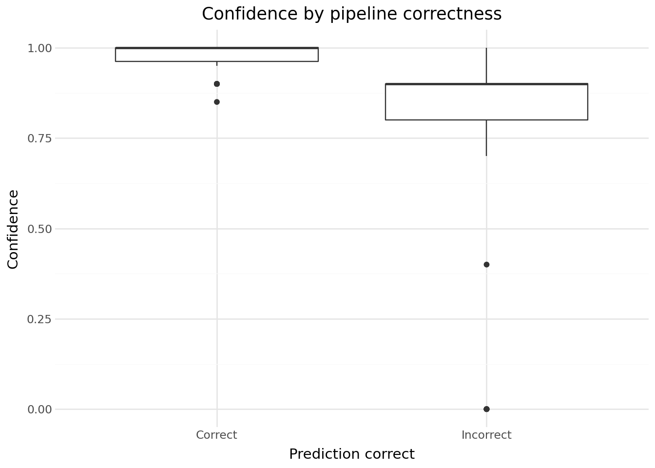
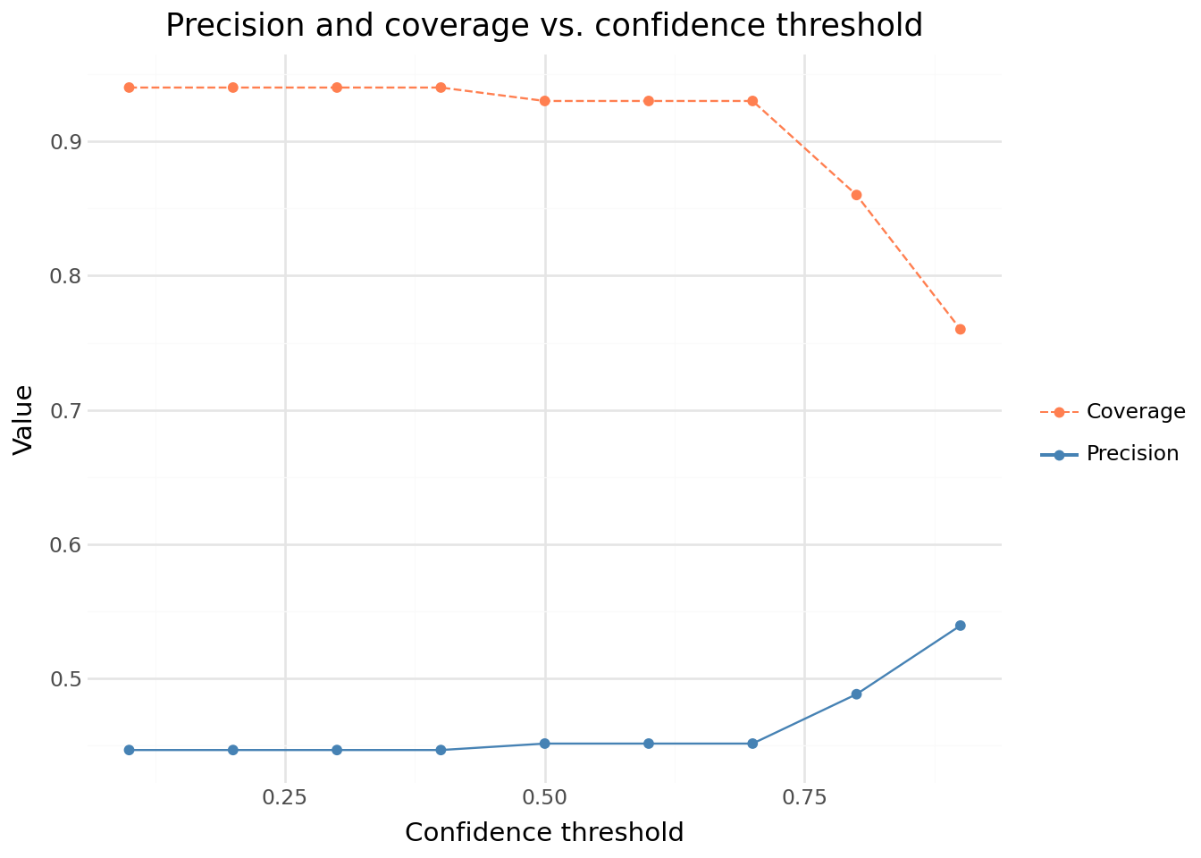
5.1 Precision–coverage trade-off

The LLM returns a confidence score. Filtering on it raises precision but lowers coverage (more labels left for manual review).

from plotnine import (
    ggplot, aes, geom_boxplot, geom_line, geom_point,
    scale_color_manual, scale_linetype_manual, labs, theme_minimal,
)

results_plot = results.assign(
    correctness=results["pipeline_correct"].map({False: "Incorrect", True: "Correct"})
)

p1 = (
    ggplot(results_plot, aes(x="correctness", y="confidence"))
    + geom_boxplot()
    + labs(title="Confidence by pipeline correctness", x="Prediction correct", y="Confidence")
    + theme_minimal()
)

rows = []
for t in [i / 10 for i in range(1, 10)]:
    subset = results[results["confidence"] >= t]
    if len(subset) > 0:
        rows.append({"threshold": t, "metric": "Precision", "value": subset["pipeline_correct"].mean()})
        rows.append({"threshold": t, "metric": "Coverage",  "value": len(subset) / len(results)})

df_thresh = pd.DataFrame(rows, columns=["threshold", "metric", "value"])

from IPython.display import display
display(p1)

if df_thresh.empty:
    print("No confidence threshold yielded a non-empty subset; skipping precision/coverage plot.")
else:
    p2 = (
        ggplot(df_thresh, aes(x="threshold", y="value", color="metric", linetype="metric"))
        + geom_line() + geom_point()
        + scale_color_manual(values={"Precision": "steelblue", "Coverage": "coral"})
        + scale_linetype_manual(values={"Precision": "solid", "Coverage": "dashed"})
        + labs(title="Precision and coverage vs. confidence threshold",
               x="Confidence threshold", y="Value", color="", linetype="")
        + theme_minimal()
    )
    display(p2)

Important

Optimistic numbers. The evaluation dataset is synthetic: clean, unambiguous one-liners generated by an LLM. Real production labels are shorter, noisier, and more ambiguous, so these figures are an upper bound on what to expect in production.

1 Goal of this tutorial

1.1 Why RAG for recodification?

1.2 What this notebook covers

2 Technical requirements

2.1 Services

2.2 Credentials

2.2.1 Getting your llm.lab API key

2.2.2 Getting your Qdrant credentials

2.3 Loading credentials in Python

3 Build the vector database

3.1 Connections

3.2 Load the NACE 2.1 nomenclature

3.3 NaceDocument: clean text + embedding + Qdrant point

3.4 Create the Qdrant collection

3.5 Embed every entry and upload to Qdrant

4 Run the RAG pipeline

4.1 Global parameters and prompt

4.2 Pipeline function

4.3 Load the evaluation dataset

4.4 Batch inference on the sample

5 Evaluation

5.1 Precision–coverage trade-off

3.3 `NaceDocument`: clean text + embedding + Qdrant point