Now that we have trained and evaluated a Random Forest model, we will train a Gradient Boosting model on the same data. We will cover the theoretical background, train a baseline model, understand the key hyperparameters, and tune them following a simple validation procedure.
An Insee working document on ensemble methods is available here. If you are unfamiliar with gradient boosting, we recommend reading it before proceeding.
1 Concepts of Gradient Boosting
Like Random Forests, Gradient Boosting is an ensemble method that combines many decision trees. However, the two methods differ fundamentally in how those trees are built and combined.
Random Forests build trees independently and in parallel, then average their predictions. Their strength comes from reducing variance through aggregation of decorrelated trees. By construction, they are quite robust to overfitting.
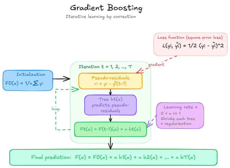
Gradient Boosting builds trees sequentially: each new tree is trained to correct the prediction errors — the pseudo-residuals — left by all previous trees. Formally, at each iteration \(t\) the model is updated as:
\[F_t(x) = F_{t-1}(x) + \eta \cdot f_t(x)\]
where \(f_t\) is the new tree and \(\eta \in (0, 1]\) is the learning rate, which scales down the contribution of each tree to avoid overreacting to individual observations.
This sequential construction gives gradient boosting a stronger capacity to reduce bias — it can fit complex relationships that a random forest might miss. In a regression problem with squared-error loss, the pseudo-residual for observation \(i\) is simply \(y_i - \hat{y}_i^{(t-1)}\): each tree literally predicts what the current model got wrong.
Overview of the Gradient Boosting training
WarningGradient boosting and overfitting
Unlike random forests, gradient boosting contains no built-in mechanism to limit overfitting. It is designed to approximate the training data as precisely as possible — including its noise. As the number of trees grows, the model increasingly captures random fluctuations in the training set rather than the true signal.
Controlling overfitting is therefore the central challenge when training a gradient boosting model, and it is the main purpose of its regularisation hyperparameters (see Section 3).
scikit-learn’s HistGradientBoostingRegressor is a histogram-based implementation, similar in spirit to LightGBM. It discretises continuous features into bins before constructing trees, making it significantly faster than the classic GradientBoostingRegressor, especially on large datasets. It also natively handles missing values without any imputation step.
For more information, you can read the detailed presentation of the gradient boosting algorithm here and the usage guide here.
2 Training a baseline Gradient Boosting model
To allow for comparison with the random forest section, we chose to use the same conditions : dropping the trans_date and prop_type features and working with the non transformed target (i.e.price per square meter) and not use the transformed target (i.e. log of the price per square meter) defined at the end of the pre-processing. We will come back to this later on and chain it with the preprocessing steps.
2.1 Exercice 7: Train your first Gradient Boosting model
Using the HistGradientBoostingRegressor class and its scikit-learn documentation page, define and train a baseline model with default hyperparameters using the same training set X_train and y_train defined in the preprocessing section.
Note: Just like for RandomForestRegressor, all parameters have default values — you do not need to pass any argument to get a working model.
See the solution
from sklearn.ensemble import HistGradientBoostingRegressorX = df.drop(columns=["price_sqm", "trans_date", "prop_type"]) y = df["price_sqm"]X_train, X_test, y_train, y_test = train_test_split( X, y, test_size=0.2, random_state=RANDOM_STATE)gb_baseline = HistGradientBoostingRegressor(random_state=RANDOM_STATE)gb_baseline.fit(X_train, y_train)
Compute the three evaluation metrics — RMSE, MAE and R² — on both the training set and the test set. Compare both sets of scores: what do you observe?
Note: Computing metrics on the training set alongside the test set is important with gradient boosting because it reveals whether the model is overfitting.
How does the default Gradient Boosting model compare with the best Random Forest model from Exercise 6?
2.2 Key Hyperparameters of Gradient Boosting
The gradient boosting algorithm has many hyperparameters, but the literature identifies a small set that most strongly influence model performance. Gradient-boosting hyperparameters are also coupled, so we cannot set them one after the other anymore. The important hyperparameters are max_iter, learning_rate, and max_depth or max_leaf_nodes (as previously discussed random forest). We recommend reading the scikit-learn MOOC on tuning here for more details. Here for this tutorial, we focus on these four groups:
1. Number of trees (max_iter)
max_iter, similarly to the n_estimators hyperparameter in random forests, controls the number of trees in the final estimator. With gradient boosting, if you add a tree, you will get closer to the target. Unlike a random forest, the performance of a gradient boosting model on the training set grows continuously as more trees are added — it never plateaus. But if the number of trees is too large, the model will overfit : your score on the training set will get close to 100% but the score on the test set will not increase. If the number of trees is too small, the model will underfit. The optimal number of trees therefore depends on the learning rate: a lower learning rate requires more trees to achieve equivalent performance.
In HistGradientBoostingRegressor, the number of trees is controlled by max_iter (default: 100).
As a reminder, overfitting occurs when a model captures statistical noise and idiosyncrasies of the training data. This information should not influence the model’s predictions on new data (i.e., during inference). Conversely, underfitting occurs when a model is too simple to capture the underlying patterns in the data, resulting in poor performance on both training and unseen data.
2. Tree complexity (max_leaf_nodes, max_depth)
These parameters control the complexity of each individual tree (the weak learner). max_leaf_nodes sets the maximum number of terminal leaves; max_depth sets the maximum depth. Shallow trees (few leaves, low depth) reduce overfitting but limit the ability of each tree to capture interactions between variables. Deeper trees are more expressive but risk overfitting and slow down training. In gradient boosting, trees are typically kept shallow (typically between 3 to 8 levels, equivalent to 8 (2^3) to 256 (2^8) leaves ) — the model’s power comes from combining many of them, not from the complexity of each one. Therefore, it can be beneficial to increase max_iter if max_depth is low.
In HistGradientBoostingRegressor, the leaf-wise growth strategy is used, making max_leaf_nodes the primary parameter (default: 31).
3. Learning rate (learning_rate)
The learning rate \(\eta \in (0, 1]\) scales the contribution of each tree to the ensemble. A lower value makes learning more gradual — each tree corrects errors more cautiously — which typically reduces overfitting but requires more trees to converge. A higher value speeds up training but can cause instability and overfitting. Typical values range from 0.01 to 0.3. The learning rate and the number of trees are tightly linked.
In HistGradientBoostingRegressor, the default learning-rate is 0.1.
l2_regularization: applies an L2 penalty to the leaf weights, shrinking them towards zero. This reduces the influence of outliers and limits overfitting.
In HistGradientBoostingRegressor, default value is 0 (no regularisation), but a positive value is often recommended in practice.
min_samples_leaf: the minimum number of observations that a terminal leaf must contain. Higher values prevent the model from creating very small leaves and thus from overfitting.
In HistGradientBoostingRegressor, default value is 20.
We follow the iterative simple validation procedure described in the usage guide. Rather than using cross-validation (which would require training many models), we evaluate each hyperparameter configuration once on the test set and proceed in three sequential steps:
Jointly optimise the number of trees and the learning rate — these two hyperparameters are tightly linked and must be tuned together.
Jointly optimise the tree structure — using the best values from step 1.
Optimise the regularisation parameters — using the best values from steps 1 and 2.
For each step, we record both training and test scores to monitor overfitting. A large gap between train and test performance signals that the model is overfitting.
Note
We use the same X_train, X_test, y_train, y_test splits defined in the preprocessing section. Note that strictly speaking, the test set should not be used to select hyperparameters — a proper hold-out validation set should be used instead. We use the test set here for simplicity and pedagogical clarity.
For convenience, we prepare the data and pipeline with the following instructions :
Drop the features prop_type, trans_date of the dataframe;
Create X dataframe and y Pandas Serie for training our model on prices per square meters.
Define the new training and testing datasets X_train, X_test, y_train, y_test.
Update the definition of our previous pipeline structure (with TransformedTargetRegressor) with a Gradient Boosting model with random state and early stopping parameters.
Note : We will tune the hyperparameters using the whole pipeline and this set of training and test sets.
2.4.1 Step 1 — Jointly optimise the number of trees and the learning rate
Define the parameter grid for max_iter and learning_rate, then run a GridSearchCV with 2 folds (to speed-up training time), scoring="r2" and return_train_score=True. Use n_jobs=-1 to parallelise the search.
The grid search can take some time to compute (for example, about 40 minutes for 36 iterations) so don’t choose max_iter above 1000 and more than 2 and 2 sets of values.
Be careful : usually, you have to choose more than 2 folds for the cross validation (often 5)
TipHint
When using GridSearchCV, the parameter names must match those of the estimator passed to it. Here we pass a HistGradientBoostingRegressor directly, so names are simply max_iter and learning_rate.
To retrieve all fold scores after fitting, use cv_results_ — it is a dict that contains mean_train_score, mean_test_score, and the corresponding parameter values.
Make it a function called results_to_df which takes as input the cross-validation results and returns a dataframe, sorted by descending validation R² values . For that :
Retrieve the cross-validation results as a DataFrame;
Display the mean train and validation R² for each combination, sorted by descending validation R².
TipHint
The cross-validation results are available through the model’s cv_results_ attribute. All parameters names are prefixed with param_regressor__GB__. The metrics we are looking for are suffixed mean_train_score and mean_test_score.
See the solution
def results_to_df(results_: dict): pattern ="param_regressor__GB__" pattern_len=len(pattern) params = [key for key in results_.keys() if key.startswith(pattern)] matching_keys = params + ["mean_train_score", "mean_test_score"] rename_params = {key: key[pattern_len:] for key in params} rename_params["mean_train_score"] ="train_r2" rename_params["mean_test_score"] ="val_r2" results_df_ = pd.DataFrame(results_)[matching_keys].rename(columns=rename_params)return results_df_.sort_values("val_r2", ascending=False)df_step1 = results_to_df(gs_step1.cv_results_)
Important
In scikit-learn’s GridSearchCV, the column mean_test_score refers to the cross-validation score computed on the held-out fold at each split — not to a score on X_test. The naming can be confusing: “test” here means “not used for training this fold”. To avoid ambiguity we rename this column val_r2 in the results DataFrame.
Plot the mean train and validation R² on a single plot, with one line per learning_rate. Make it a function called def plot_results_cv which takes as input the hyperparameter to put on the X axis and the results as a dataframe from previous function.
What do you observe about the interplay between the two hyperparameters?
What value for the learning rate and the number of tree do you chose, taking into consideration computation efficiency ?
See the solution
import matplotlib.pyplot as pltdef plot_results_cv(param_x:str, results_df_): param_group_by = [column for column in results_df_.columns.to_list() if column notin [param_x, "val_r2", "train_r2"]][0] param_group_by_values = results_df_[param_group_by].unique() fig, ax = plt.subplots(figsize=(13, 4))for param_line in param_group_by_values: subset = results_df_[results_df_[param_group_by] == param_line].sort_values(param_x) line, = ax.plot(subset[param_x], subset["train_r2"], linestyle="--", marker="o", label=f"Train {param_group_by}={param_line}") ax.plot(subset[param_x], subset["val_r2"], marker="x", color=line.get_color(), label=f"Val {param_group_by}={param_line}") ax.set_xlabel(f"{param_x}") ax.set_ylabel("R²") ax.set_title(f"Joint optimisation of {param_group_by} and {param_x}") ax.legend(fontsize=8) ax.grid(True, linestyle=":") plt.tight_layout() plt.show()plot_results_cv("max_iter", df_step1)
If the best value of max_iter is the largest value tested (1000), consider extending the grid before moving to the next step.
See the solution
BEST_ITER =500# to automatically catch the best hyperparameter, set to : gs_step1.best_params_["regressor__GB__max_iter"]BEST_LR =0.2# to automatically catch the best hyperparameter, set to : gs_step1.best_params_["regressor__GB__learning_rate"]
2.4.2 Step 2 — Jointly optimise the tree structure
Fix max_iter and learning_rate to the best values found in step 1, then run a second GridSearchCV over max_depth and min_samples_leaf with other settings unchanged.
2.4.3 Step 3 — Optimise the regularisation parameters
Using the best hyperparameters found in steps 1 and 2, train one model for each value of l2_regularization in [0.0, 0.1, 0.3, 0.5, 1.0]. To use our predefined function, make it as if it was a cross validation with max_iter set to the above chosen value. Using our pre-defined function, plot the result.
Does regularisation help reduce the gap between train and test performance?
Train the final HistGradientBoostingRegressor using all the best hyperparameters identified in the previous steps. Then re-train it on the full training set.
See the solution
gb_final = HistGradientBoostingRegressor( max_iter=BEST_ITER, learning_rate=BEST_LR, max_depth=BEST_DEPTH, min_samples_leaf=BEST_MIN_LEAF, l2_regularization=BEST_L2, random_state=RANDOM_STATE,)X = df.drop(columns=["price_sqm"])y = df["price_sqm"] X_train, X_test, y_train, y_test = train_test_split( X, y, test_size=0.2, random_state=RANDOM_STATE)# Wrap in the same pipeline / TransformedTargetRegressor as the RF sectiongb_pipeline_best = Pipeline([ ("preprocessor", preprocessor), # same preprocessor as defined in the preprocessing section ("GB", gb_final),])gb_model_final = TransformedTargetRegressor( regressor=gb_pipeline_best, transformer=y_transformer # same targettransformer as defined in preprocessing section)gb_model_final.fit(X_train, y_train)print("Final model trained.")
3 Exercice 9: Evaluate the final Gradient Boosting model
Now that the model has been tuned, evaluate its performance on the test set and compare it to the Random Forest baseline.
Compute RMSE, MAE and R² on both the training and test sets for the final gradient boosting model using our print_metrics function.
See the solution
model = gb_model_bestlist= [("train", X_train, y_train), ("test", X_test, y_test)]for split, X, y inlist: print_metrics(model, split, X, y)
Plot predicted values against actual values on the test set.
See the solution
import matplotlib.pyplot as plty_pred_test = gb_model_best.predict(X_test)fig, ax = plt.subplots(figsize=(7, 7))ax.scatter(y_test, y_pred_test, alpha=0.3, s=5, label="Predictions")lims = [min(y_test.min(), y_pred_test.min()),max(y_test.max(), y_pred_test.max())]ax.plot(lims, lims, "r--", linewidth=1.5, label="Perfect prediction")ax.set_xlabel("Actual values")ax.set_ylabel("Predicted values")ax.set_title("Predicted vs. Actual values on the test set\n(Gradient Boosting)")ax.legend()plt.tight_layout()plt.show()
Congrats 🎉! You have successfully trained, tuned, and evaluated a Gradient Boosting model and compared it to the Random Forest baseline.