Data acquisition

1 Sentinel-2 Images

This section describes how Sentinel-2 images are retrieved, visualised, and organised for model training.

1.1 What is Sentinel-2?

Sentinel-2 is an Earth observation mission from the European Space Agency (ESA), part of the Copernicus programme. It consists of two twin satellites — Sentinel-2A and Sentinel-2B — placed in the same sun-synchronous orbit but phased 180 degrees apart, giving a 5-day revisit time at the equator.

Key characteristics:

13 spectral bands spanning visible, near-infrared (NIR) and short-wave infrared (SWIR)
Spatial resolution of 10 m, 20 m or 60 m depending on the band
290 km swath width
Free and open data policy

These properties make Sentinel-2 a reference dataset for land-cover mapping, agricultural monitoring, forestry, urban change detection and many other applications.

1.1.1 Spectral bands

Band	Central wavelength (nm)	Resolution (m)	Description
B1	443	60	Coastal aerosol
B2	490	10	Blue
B3	560	10	Green
B4	665	10	Red
B5	705	20	Vegetation red edge
B6	740	20	Vegetation red edge
B7	783	20	Vegetation red edge
B8	842	10	NIR
B8A	865	20	Narrow NIR
B9	945	60	Water vapour
B10	1375	60	SWIR – Cirrus
B11	1610	20	SWIR
B12	2190	20	SWIR

1.2 Copernicus Data Space Ecosystem (CDSE) — Sentinel Hub API

The official programmatic access point for Sentinel-2 data is the Sentinel Hub API, part of the Copernicus Data Space Ecosystem (CDSE). It provides two main endpoints:

Catalog API — search for available Sentinel-2 products by area, date, and cloud cover
Processing API — download imagery on-the-fly with custom band combinations and formats

To use the Sentinel Hub API you need a free CDSE account — register at https://dataspace.copernicus.eu/. Then, register an OAuth client in the CDSE dashboard to obtain a Client ID and Client Secret.

1.2.1 Authentication

Sentinel Hub uses OAuth2 client credentials. Authenticate with oauthlib and requests_oauthlib:

from oauthlib.oauth2 import BackendApplicationClient
from requests_oauthlib import OAuth2Session

client_id = "your-client-id"
client_secret = "your-client-secret"

client = BackendApplicationClient(client_id=client_id)
oauth = OAuth2Session(client=client)
token = oauth.fetch_token(
    token_url="https://identity.dataspace.copernicus.eu/auth/realms/CDSE/protocol/openid-connect/token",
    client_secret=client_secret,
    include_client_id=True,
)

1.2.2 Searching the catalogue

Use the Catalog API to find Sentinel-2 L2A products for a given area and date range:

catalog_url = "https://sh.dataspace.copernicus.eu/api/v1/catalog/1.0.0/search"

search_body = {
    "collections": ["sentinel-2-l2a"],
    "datetime": "2021-06-01T00:00:00Z/2021-06-30T23:59:59Z",
    "bbox": [23.0, 42.0, 24.0, 43.0],  # [west, south, east, north] in WGS84
    "limit": 10,
    "filter": "eo:cloud_cover < 20",
    "filter-lang": "cql2-text",
}

response = oauth.post(catalog_url, json=search_body)
results = response.json()
print(f"Found {len(results['features'])} products")

1.2.3 Downloading imagery

Use the Processing API to download a true-colour Sentinel-2 image as a GeoTIFF:

process_url = "https://sh.dataspace.copernicus.eu/api/v1/process"

evalscript = """
//VERSION=3
function setup() {
  return { input: ["B04", "B03", "B02"], output: { bands: 3, sampleType: "UINT16" } };
}
function evaluatePixel(sample) {
  return [sample.B04, sample.B03, sample.B02];
}
"""

request_body = {
    "input": {
        "bounds": {
            "bbox": [23.0, 42.0, 24.0, 43.0],
            "properties": {"crs": "http://www.opengis.net/def/crs/EPSG/0/4326"},
        },
        "data": [
            {
                "type": "sentinel-2-l2a",
                "dataFilter": {
                    "timeRange": {
                        "from": "2021-06-01T00:00:00Z",
                        "to": "2021-06-30T23:59:59Z",
                    },
                    "maxCloudCoverage": 20,
                },
            }
        ],
    },
    "output": {
        "width": 512,
        "height": 512,
        "responses": [{"identifier": "default", "format": {"type": "image/tiff"}}],
    },
    "evalscript": evalscript,
}

response = oauth.post(process_url, json=request_body)
with open("output.tif", "wb") as f:
    f.write(response.content)

collections: use "sentinel-2-l2a" for Level-2A products (surface reflectance, atmospherically corrected).
bbox: bounding box as [west, south, east, north] in WGS84 (EPSG:4326).
filter: CQL2 expression for metadata filtering, e.g. "eo:cloud_cover < 20" keeps only scenes with under 20 % cloud cover.

Exercise 1 (optional) — Query the Sentinel Hub Catalog API

Goal: Use the Sentinel Hub Catalog API to search for Sentinel-2 L2A products over Bulgaria during June 2021 with less than 10 % cloud cover.

Steps:

Authenticate with OAuth2 using OAuth2Session + BackendApplicationClient against the CDSE token endpoint
Build a Catalog API request body with collections: ["sentinel-2-l2a"], datetime, bbox covering Bulgaria, and a cloud-cover filter
POST to the Catalog API endpoint and parse the JSON response
Print the number of features found

from oauthlib.oauth2 import BackendApplicationClient
from requests_oauthlib import OAuth2Session

# Step 1: Authenticate with OAuth2
client_id = ___      # TODO: your CDSE OAuth client ID
client_secret = ___  # TODO: your CDSE OAuth client secret

client = BackendApplicationClient(client_id=client_id)
oauth = OAuth2Session(client=client)
token = oauth.fetch_token(
    token_url=___,  # TODO: CDSE token URL
    client_secret=client_secret,
    include_client_id=True,
)

# Step 2: Build the Catalog API request body
catalog_url = "https://sh.dataspace.copernicus.eu/api/v1/catalog/1.0.0/search"
search_body = {
    "collections": ___,  # TODO: ["sentinel-2-l2a"]
    "datetime": ___,     # TODO: "2021-06-01T00:00:00Z/2021-06-30T23:59:59Z"
    "bbox": ___,         # TODO: Bulgaria bounding box [west, south, east, north]
    "limit": 50,
    "filter": ___,       # TODO: CQL2 cloud cover filter
    "filter-lang": "cql2-text",
}

# Step 3: POST to the Catalog API
response = ___  # TODO: oauth.post(catalog_url, json=search_body)
results = response.json()

# Step 4: Print the number of features
print(f"Found {len(results['features'])} products")

Hint — Exercise 1

The CDSE token URL is "https://identity.dataspace.copernicus.eu/auth/realms/CDSE/protocol/openid-connect/token".
Bulgaria’s approximate bounding box in WGS84 is [22.0, 41.0, 29.0, 44.5].
Use "eo:cloud_cover < 10" as the CQL2 filter for cloud cover under 10 %.
The datetime range format is "start/end" in ISO 8601, e.g. "2021-06-01T00:00:00Z/2021-06-30T23:59:59Z".

Solution — Exercise 1

from oauthlib.oauth2 import BackendApplicationClient
from requests_oauthlib import OAuth2Session

client_id = "your-client-id"
client_secret = "your-client-secret"

client = BackendApplicationClient(client_id=client_id)
oauth = OAuth2Session(client=client)
token = oauth.fetch_token(
    token_url="https://identity.dataspace.copernicus.eu/auth/realms/CDSE/protocol/openid-connect/token",
    client_secret=client_secret,
    include_client_id=True,
)

catalog_url = "https://sh.dataspace.copernicus.eu/api/v1/catalog/1.0.0/search"
search_body = {
    "collections": ["sentinel-2-l2a"],
    "datetime": "2021-06-01T00:00:00Z/2021-06-30T23:59:59Z",
    "bbox": [22.0, 41.0, 29.0, 44.5],
    "limit": 50,
    "filter": "eo:cloud_cover < 10",
    "filter-lang": "cql2-text",
}

response = oauth.post(catalog_url, json=search_body)
results = response.json()
print(f"Found {len(results['features'])} products")

Once you have searched the catalogue, you can use the Processing API to download imagery directly, then upload it to S3 so it can be shared with your team. The SSP Cloud provides an S3-compatible object store accessible via s3fs. Here is how to initialise an S3FileSystem and upload a file:

from utils import get_file_system

fs = get_file_system()

# Upload a local file to S3
fs.put("./output.tif", "s3://my-bucket/sentinel2/output.tif")

Exercise 2 (optional) — Download a Sentinel-2 image with the Processing API and upload to S3

Goal: Use the Sentinel Hub Processing API to download a true-colour Sentinel-2 image for Bulgaria (June 2021) and upload it to your personal S3 bucket.

Steps:

Authenticate with OAuth2 (reuse the session from Exercise 1)
Build a Processing API request with bbox, time range, evalscript for true-colour RGB, and output as image/tiff
POST to the Processing API endpoint and save the response content locally
Initialise an S3FileSystem with get_file_system() and upload the file with fs.put()

from utils import get_file_system

# Step 1: Reuse the authenticated OAuth2 session from Exercise 1

# Step 2: Build the Processing API request
process_url = "https://sh.dataspace.copernicus.eu/api/v1/process"

evalscript = """
//VERSION=3
function setup() {
  return { input: ["B04", "B03", "B02"], output: { bands: 3, sampleType: "UINT16" } };
}
function evaluatePixel(sample) {
  return [sample.B04, sample.B03, sample.B02];
}
"""

request_body = {
    "input": {
        "bounds": {
            "bbox": ___,  # TODO: Bulgaria bounding box [west, south, east, north]
            "properties": {"crs": "http://www.opengis.net/def/crs/EPSG/0/4326"},
        },
        "data": [
            {
                "type": ___,  # TODO: "sentinel-2-l2a"
                "dataFilter": {
                    "timeRange": {
                        "from": ___,  # TODO: start date ISO 8601
                        "to": ___,    # TODO: end date ISO 8601
                    },
                    "maxCloudCoverage": ___,  # TODO: max cloud cover percentage
                },
            }
        ],
    },
    "output": {
        "width": 512,
        "height": 512,
        "responses": [{"identifier": "default", "format": {"type": ___}}],  # TODO: "image/tiff"
    },
    "evalscript": evalscript,
}

# Step 3: POST and save locally
response = ___  # TODO: oauth.post(process_url, json=request_body)
local_path = "bulgaria_rgb.tif"
with open(local_path, "wb") as f:
    f.write(___)  # TODO: response.content

# Step 4: Upload to S3
fs = ___  # TODO: get_file_system()
fs.put(___, ___)  # TODO: local_path, S3 destination path

Hint — Exercise 2

The Processing API URL is "https://sh.dataspace.copernicus.eu/api/v1/process".
Use [22.0, 41.0, 29.0, 44.5] for the Bulgaria bounding box.
Time range uses ISO 8601: "2021-06-01T00:00:00Z" to "2021-06-30T23:59:59Z".
Set maxCloudCoverage to 10 (integer, not a string range).
The response content (response.content) is the raw TIFF bytes — write them to a file in binary mode.
get_file_system() reads SSP Cloud credentials from environment variables.

Solution — Exercise 2

from utils import get_file_system

process_url = "https://sh.dataspace.copernicus.eu/api/v1/process"

evalscript = """
//VERSION=3
function setup() {
  return { input: ["B04", "B03", "B02"], output: { bands: 3, sampleType: "UINT16" } };
}
function evaluatePixel(sample) {
  return [sample.B04, sample.B03, sample.B02];
}
"""

request_body = {
    "input": {
        "bounds": {
            "bbox": [22.0, 41.0, 29.0, 44.5],
            "properties": {"crs": "http://www.opengis.net/def/crs/EPSG/0/4326"},
        },
        "data": [
            {
                "type": "sentinel-2-l2a",
                "dataFilter": {
                    "timeRange": {
                        "from": "2021-06-01T00:00:00Z",
                        "to": "2021-06-30T23:59:59Z",
                    },
                    "maxCloudCoverage": 10,
                },
            }
        ],
    },
    "output": {
        "width": 512,
        "height": 512,
        "responses": [{"identifier": "default", "format": {"type": "image/tiff"}}],
    },
    "evalscript": evalscript,
}

response = oauth.post(process_url, json=request_body)
local_path = "bulgaria_rgb.tif"
with open(local_path, "wb") as f:
    f.write(response.content)

fs = get_file_system()
fs.put(local_path, "s3://my-bucket/sentinel2/bulgaria_rgb.tif")

1.3 What is rasterio?

rasterio is a Python library built on top of GDAL for reading and writing geospatial raster data (GeoTIFF, etc.). It is the standard tool for working with satellite imagery in Python.

Key concepts:

Raster = a grid of pixels organised into bands (layers). Each band represents one channel of data (e.g. a spectral band from a satellite sensor).
rasterio.open(path) returns a DatasetReader — works with local files and HTTPS URLs alike.
src.read(bands) returns a NumPy array with shape (bands, H, W). Band indices are 1-based: band 1 is the first band, not band 0.
src.crs — the coordinate reference system attached to the raster.
src.bounds — the geographic extent as (left, bottom, right, top).
src.profile / src.meta — full metadata dictionary (driver, dtype, nodata value, affine transform, etc.).

Why band indexing matters: Sentinel-2 images have 13 spectral bands (see the table above). Reading specific band combinations reveals different features:

src.read([4, 3, 2]) → true-colour RGB (Red, Green, Blue)
src.read([8, 4, 3]) → false-colour composite (NIR, Red, Green) — vegetation appears bright red
src.read([8, 4]) → bands needed for NDVI (Normalised Difference Vegetation Index)

You will practise these combinations in the exercises below.

2 Accessing pre-processed patches

For this project, pre-processed Sentinel-2 patches are publicly available on the SSP Cloud object storage. You can access them directly over HTTPS — no authentication or special tools required.

The URL follows this pattern:

https://minio.lab.sspcloud.fr/projet-hackathon-ntts-2025/data-preprocessed/patchs/CLCplus-Backbone/SENTINEL2/{NUTS}/{year}/{size}/{patch_id}.tif

Each pre-processed patch is a GeoTIFF covering a 250 x 250 pixel area (2 500 m at 10 m resolution). The URL path encodes the key metadata:

.../SENTINEL2/{NUTS}/{year}/{size}/{xmin}_{ymin}_{idx}_{id}.tif

Field	Example value	Meaning
NUTS	`FRJ27`	NUTS-3 region (Haute-Garonne, near Toulouse)
year	`2018`	Acquisition year
size	`250`	Tile size in pixels
xmin, ymin	`3649890, 2331750`	Lower-left corner in EPSG:3035 (metres)

rasterio can open these URLs directly, just like local files:

import rasterio
import numpy as np

tile_url = (
    "https://minio.lab.sspcloud.fr/projet-hackathon-ntts-2025/"
    "data-preprocessed/patchs/CLCplus-Backbone/SENTINEL2/"
    "FRJ27/2018/250/3649890_2331750_0_937.tif"
)

with rasterio.open(tile_url) as src:
    tile_crs = src.crs
    tile_bounds = src.bounds
    tile_count = src.count
    tile_height = src.height
    tile_width = src.width
    # Read RGB bands: B4 (Red), B3 (Green), B2 (Blue)
    rgb_data = src.read([4, 3, 2])

print(f"CRS:    {tile_crs}")
print(f"Bounds: {tile_bounds}")
print(f"Shape:  {tile_count} bands x {tile_height} x {tile_width} px")

CRS:    EPSG:3035
Bounds: BoundingBox(left=3649890.0, bottom=2331750.0, right=3652390.0, top=2334250.0)
Shape:  14 bands x 250 x 250 px

Now let’s display the tile as an RGB composite (true-colour: Red, Green, Blue):

import matplotlib.pyplot as plt

# Transpose to (H, W, 3) and normalize for display
rgb = np.transpose(rgb_data, (1, 2, 0)).astype(np.float32)
p98 = np.percentile(rgb, 98)
rgb = np.clip(rgb / p98, 0, 1)

fig, ax = plt.subplots(figsize=(5, 5))
ax.imshow(rgb)
ax.set_title("Sentinel-2 RGB composite (B4, B3, B2) — FRJ27")
ax.axis("off")
plt.tight_layout()
plt.show()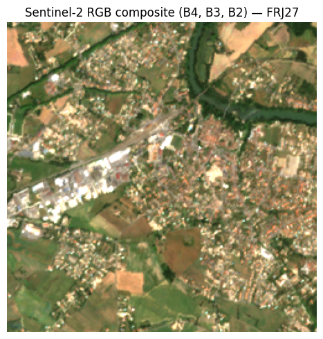

Exercise 3 — Read a Sentinel-2 tile and display it

Goal: Open a different pre-processed Sentinel-2 patch via its HTTPS URL, extract the RGB bands, normalize the image, and display it.

Steps:

Open the tile with rasterio.open(tile_url) and read bands 4, 3, 2 (Red, Green, Blue)
Store the CRS and bounds from the rasterio source
Transpose the array to (H, W, 3) and normalize for display (divide by the 98th percentile, clip to [0, 1])
Display the RGB composite with matplotlib

import rasterio
import numpy as np
import matplotlib.pyplot as plt

tile_url = (
    "https://minio.lab.sspcloud.fr/projet-hackathon-ntts-2025/"
    "data-preprocessed/patchs/CLCplus-Backbone/SENTINEL2/"
    "FRJ27/2018/250/3649890_2331750_0_937.tif"
)

# Step 1: Open the tile and read RGB bands (4, 3, 2)
with rasterio.open(tile_url) as src:
    rgb_data = ___  # TODO: read bands 4, 3, 2
    tile_crs = ___  # TODO
    tile_bounds = ___  # TODO

# Step 2: Transpose to (H, W, 3) and normalize
rgb = ___  # TODO: np.transpose, then normalize with 98th percentile and clip

# Step 3: Display
fig, ax = plt.subplots(figsize=(5, 5))
___  # TODO: ax.imshow(...)
ax.set_title("Sentinel-2 RGB composite")
ax.axis("off")
plt.tight_layout()
plt.show()

Hint — Exercise 3

Inside the with rasterio.open(tile_url) as src: block, use src.read([4, 3, 2]) to get a (3, H, W) array.
src.crs and src.bounds give you the CRS and bounding box.
Transpose with np.transpose(rgb_data, (1, 2, 0)), cast to float32, then normalize: divide by np.percentile(rgb, 98) and clip to [0, 1] with np.clip.

Solution — Exercise 3

import rasterio
import numpy as np
import matplotlib.pyplot as plt

tile_url = (
    "https://minio.lab.sspcloud.fr/projet-hackathon-ntts-2025/"
    "data-preprocessed/patchs/CLCplus-Backbone/SENTINEL2/"
    "FRJ27/2018/250/3649890_2331750_0_937.tif"
)

with rasterio.open(tile_url) as src:
    rgb_data = src.read([4, 3, 2])
    tile_crs = src.crs
    tile_bounds = src.bounds

rgb = np.transpose(rgb_data, (1, 2, 0)).astype(np.float32)
p98 = np.percentile(rgb, 98)
rgb = np.clip(rgb / p98, 0, 1)

fig, ax = plt.subplots(figsize=(5, 5))
ax.imshow(rgb)
ax.set_title("Sentinel-2 RGB composite")
ax.axis("off")
plt.tight_layout()
plt.show()

Exercise 4 — Explore raster metadata and create a false-colour composite

Goal: Inspect the raster metadata of a Sentinel-2 tile using src.profile, then create a false-colour composite using bands 8 (NIR), 4 (Red), 3 (Green). In this composite, vegetation appears bright red because it reflects strongly in the near-infrared.

Steps:

Open the tile with rasterio.open(tile_url) and print src.profile
Read bands [8, 4, 3] (NIR, Red, Green)
Normalize the false-colour image (same method as Exercise 3: 98th percentile + clip)
Display the true-colour RGB (from Exercise 3) and false-colour composite side by side

import rasterio
import numpy as np
import matplotlib.pyplot as plt

tile_url = (
    "https://minio.lab.sspcloud.fr/projet-hackathon-ntts-2025/"
    "data-preprocessed/patchs/CLCplus-Backbone/SENTINEL2/"
    "FRJ27/2018/250/3649890_2331750_0_937.tif"
)

# Step 4a: Open the tile and print the raster profile
with rasterio.open(tile_url) as src:
    print(___) # TODO: print src.profile

    # Step 4b: Read false-colour bands (NIR=8, Red=4, Green=3)
    fc_data = ___  # TODO: src.read([8, 4, 3])

# Step 4c: Normalize for display
fc = np.transpose(fc_data, (1, 2, 0)).astype(np.float32)
p98 = ___  # TODO: np.percentile(fc, 98)
fc = ___   # TODO: np.clip(fc / p98, 0, 1)

# Step 4d: Display side by side with the true-colour RGB
fig, axes = plt.subplots(1, 2, figsize=(10, 5))
axes[0].imshow(rgb)
axes[0].set_title("True colour (B4, B3, B2)")
axes[0].axis("off")
___  # TODO: axes[1].imshow(fc)
axes[1].set_title("False colour (B8, B4, B3)")
axes[1].axis("off")
plt.tight_layout()
plt.show()

Hint — Exercise 4

src.profile is a dictionary — just print(src.profile) to see driver, dtype, crs, transform, etc.
src.read([8, 4, 3]) reads NIR, Red, Green in that order → shape (3, H, W).
Normalize exactly as in Exercise 3: transpose to (H, W, 3), divide by np.percentile(fc, 98), clip to [0, 1].

Solution — Exercise 4

import rasterio
import numpy as np
import matplotlib.pyplot as plt

tile_url = (
    "https://minio.lab.sspcloud.fr/projet-hackathon-ntts-2025/"
    "data-preprocessed/patchs/CLCplus-Backbone/SENTINEL2/"
    "FRJ27/2018/250/3649890_2331750_0_937.tif"
)

with rasterio.open(tile_url) as src:
    print(src.profile)
    fc_data = src.read([8, 4, 3])

fc = np.transpose(fc_data, (1, 2, 0)).astype(np.float32)
p98 = np.percentile(fc, 98)
fc = np.clip(fc / p98, 0, 1)

fig, axes = plt.subplots(1, 2, figsize=(10, 5))
axes[0].imshow(rgb)
axes[0].set_title("True colour (B4, B3, B2)")
axes[0].axis("off")
axes[1].imshow(fc)
axes[1].set_title("False colour (B8, B4, B3)")
axes[1].axis("off")
plt.tight_layout()
plt.show()

Exercise 5 — Compute and display NDVI

Goal: Compute the Normalised Difference Vegetation Index (NDVI) from a Sentinel-2 tile and display it as a colour-coded map.

NDVI is defined as:

\[ \text{NDVI} = \frac{\text{NIR} - \text{Red}}{\text{NIR} + \text{Red}} \]

NDVI values range from −1 to +1:

Near +1 → dense, healthy vegetation
Near 0 → bare soil, urban areas
Negative → water bodies

Steps:

Read bands 8 (NIR) and 4 (Red) as float32
Compute NDVI pixel-wise, handling division by zero
Display with imshow(cmap="RdYlGn", vmin=-1, vmax=1) and a colorbar

import rasterio
import numpy as np
import matplotlib.pyplot as plt

tile_url = (
    "https://minio.lab.sspcloud.fr/projet-hackathon-ntts-2025/"
    "data-preprocessed/patchs/CLCplus-Backbone/SENTINEL2/"
    "FRJ27/2018/250/3649890_2331750_0_937.tif"
)

# Step 5a: Read NIR (band 8) and Red (band 4) as float32
with rasterio.open(tile_url) as src:
    nir = ___  # TODO: src.read(8).astype(np.float32)
    red = ___  # TODO: src.read(4).astype(np.float32)

# Step 5b: Compute NDVI (handle division by zero)
ndvi = ___  # TODO: np.where(nir + red == 0, 0, (nir - red) / (nir + red))

# Step 5c: Display
fig, ax = plt.subplots(figsize=(6, 5))
im = ___  # TODO: ax.imshow(ndvi, cmap="RdYlGn", vmin=-1, vmax=1)
ax.set_title("NDVI — FRJ27 (2018)")
ax.axis("off")
___  # TODO: fig.colorbar(im, ax=ax, shrink=0.8, label="NDVI")
plt.tight_layout()
plt.show()

Hint — Exercise 5

src.read(8) reads a single band → shape (H, W). Cast to float32 for division.
Use np.where(nir + red == 0, 0, (nir - red) / (nir + red)) to avoid division by zero.
cmap="RdYlGn" gives a red-yellow-green colour scale: red for low NDVI, green for high.
fig.colorbar(im, ax=ax, shrink=0.8, label="NDVI") adds a colour legend.

Solution — Exercise 5

import rasterio
import numpy as np
import matplotlib.pyplot as plt

tile_url = (
    "https://minio.lab.sspcloud.fr/projet-hackathon-ntts-2025/"
    "data-preprocessed/patchs/CLCplus-Backbone/SENTINEL2/"
    "FRJ27/2018/250/3649890_2331750_0_937.tif"
)

with rasterio.open(tile_url) as src:
    nir = src.read(8).astype(np.float32)
    red = src.read(4).astype(np.float32)

ndvi = np.where(nir + red == 0, 0, (nir - red) / (nir + red))

fig, ax = plt.subplots(figsize=(6, 5))
im = ax.imshow(ndvi, cmap="RdYlGn", vmin=-1, vmax=1)
ax.set_title("NDVI — FRJ27 (2018)")
ax.axis("off")
fig.colorbar(im, ax=ax, shrink=0.8, label="NDVI")
plt.tight_layout()
plt.show()

3 Geo-manipulation with GeoPandas

Satellite imagery is inherently geospatial. Before diving into machine-learning pipelines, it is important to know how to manipulate geographic data. GeoPandas extends pandas with geometry support, making CRS transforms, spatial joins, and plotting straightforward.

3.1 Coordinate Reference Systems

Every raster and vector dataset is tied to a coordinate reference system (CRS) that defines how coordinates map to locations on Earth. The two CRS you will encounter most often in this project are:

CRS	EPSG Code	Units	Use case
WGS 84	4326	Degrees (lat/lon)	GPS, web maps, bounding-box queries
ETRS89-LAEA	3035	Metres	European statistical grids, CLC+ patches

Converting between them is a one-liner with GeoPandas:

import geopandas as gpd
from shapely.geometry import box

# Create a GeoDataFrame with the tile extent in EPSG:3035
tile_geom = box(*tile_bounds)
gdf = gpd.GeoDataFrame({"tile": ["FRJ27"]}, geometry=[tile_geom], crs="EPSG:3035")

print("EPSG:3035 bounds:")
print(gdf.total_bounds)

# Convert to WGS84 (latitude/longitude)
gdf_wgs84 = gdf.to_crs("EPSG:4326")
print("\nEPSG:4326 bounds:")
print(gdf_wgs84.total_bounds)

EPSG:3035 bounds:
[3649890. 2331750. 3652390. 2334250.]

EPSG:4326 bounds:
[ 1.66386725 43.75893034  1.6979368  43.78382633]

3.2 Building geometries from tile metadata

The patch filename encodes the lower-left corner coordinates. Combined with the tile size (2 500 m), you can reconstruct the bounding box and create a shapely geometry:

patch_filename = "3649890_2331750_0_937.tif"
parts = patch_filename.replace(".tif", "").split("_")
xmin, ymin = int(parts[0]), int(parts[1])
tile_size_m = 2500  # 250 px x 10 m/px

xmax = xmin + tile_size_m
ymax = ymin + tile_size_m

tile_box = box(xmin, ymin, xmax, ymax)
print(f"Bounding box (EPSG:3035): [{xmin}, {ymin}, {xmax}, {ymax}]")
print(f"Shapely geometry: {tile_box}")

Bounding box (EPSG:3035): [3649890, 2331750, 3652390, 2334250]
Shapely geometry: POLYGON ((3652390 2331750, 3652390 2334250, 3649890 2334250, 3649890 2331750, 3652390 2331750))

3.3 Working with GeoDataFrames

In practice, you can build a GeoDataFrame directly from rasterio metadata — no filename parsing needed:

tile_gdf = gpd.GeoDataFrame(
    {"tile": ["FRJ27"], "year": [2018]},
    geometry=[box(*tile_bounds)],
    crs=tile_crs,
)
tile_gdf

	tile	year	geometry
0	FRJ27	2018	POLYGON ((3652390 2331750, 3652390 2334250, 36...

3.4 Overlaying boundaries on images

Combining a raster image with vector boundaries is a common operation. Use imshow with the extent parameter to position the image in coordinate space, then overlay the GeoDataFrame boundary:

fig, ax = plt.subplots(figsize=(6, 6))
extent = [tile_bounds.left, tile_bounds.right, tile_bounds.bottom, tile_bounds.top]
ax.imshow(rgb, extent=extent)
tile_gdf.boundary.plot(ax=ax, color="red", linewidth=2)
ax.set_xlabel("Easting (m)")
ax.set_ylabel("Northing (m)")
ax.set_title("Sentinel-2 tile with boundary overlay (EPSG:3035)")
plt.tight_layout()
plt.show()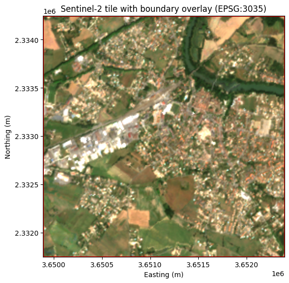

Exercise 6 — Build a GeoDataFrame from tile bounds and convert CRS

Goal: Create a GeoDataFrame from the tile’s bounding box, then convert it from EPSG:3035 to EPSG:4326 (WGS84). Print the bounds in both CRS.

Steps:

Create a shapely.geometry.box from tile_bounds
Build a GeoDataFrame with that geometry and crs="EPSG:3035"
Convert to EPSG:4326 using .to_crs()
Print total_bounds in both CRS

import geopandas as gpd
from shapely.geometry import box

# Step 1: Create a box geometry from tile_bounds
tile_geom = ___  # TODO: box(*tile_bounds)

# Step 2: Build a GeoDataFrame in EPSG:3035
gdf = ___  # TODO: gpd.GeoDataFrame(...)

# Step 3: Convert to WGS84
gdf_wgs84 = ___  # TODO: gdf.to_crs(...)

# Step 4: Print bounds in both CRS
print("EPSG:3035 bounds:", gdf.total_bounds)
print("EPSG:4326 bounds:", gdf_wgs84.total_bounds)

Hint — Exercise 6

box(*tile_bounds) unpacks (left, bottom, right, top) into a rectangular polygon.
gpd.GeoDataFrame({"tile": ["FRJ27"]}, geometry=[tile_geom], crs="EPSG:3035") creates the GeoDataFrame.
.to_crs("EPSG:4326") reprojects to latitude/longitude.

Solution — Exercise 6

import geopandas as gpd
from shapely.geometry import box

tile_geom = box(*tile_bounds)
gdf = gpd.GeoDataFrame({"tile": ["FRJ27"]}, geometry=[tile_geom], crs="EPSG:3035")
gdf_wgs84 = gdf.to_crs("EPSG:4326")

print("EPSG:3035 bounds:", gdf.total_bounds)
print("EPSG:4326 bounds:", gdf_wgs84.total_bounds)

Exercise 7 — Spatial join with NUTS3 regions

Goal: Identify which NUTS3 region(s) a Sentinel-2 tile intersects using a spatial join, and compute the tile’s area in km².

A spatial join (gpd.sjoin) combines two GeoDataFrames based on the geometric relationship between their features (e.g. intersects, contains, within). This is useful for linking raster tiles to administrative boundaries.

Steps:

Load NUTS3 boundaries from the Eurostat GeoJSON endpoint (EPSG:3035)
Create a GeoDataFrame for the tile (reuse tile_bounds and tile_crs from Exercise 3)
Perform a spatial join with predicate="intersects"
Print the matching NUTS_ID and NUTS_NAME
Compute the tile area in km² (tile_geom.area / 1e6)

import geopandas as gpd
from shapely.geometry import box

# Step 7a: Load NUTS3 boundaries (EPSG:3035)
nuts_url = (
    "https://gisco-services.ec.europa.eu/distribution/v2/"
    "nuts/geojson/NUTS_RG_01M_2021_3035_LEVL_3.geojson"
)
nuts = ___  # TODO: gpd.read_file(nuts_url)

# Step 7b: Create a GeoDataFrame for the tile
tile_geom = box(*tile_bounds)
tile_gdf = ___  # TODO: gpd.GeoDataFrame(..., geometry=[tile_geom], crs=tile_crs)

# Step 7c: Spatial join — find which NUTS3 regions the tile intersects
joined = ___  # TODO: gpd.sjoin(tile_gdf, nuts, predicate="intersects")

# Step 7d: Print matching regions
for _, row in joined.iterrows():
    print(f"NUTS_ID: {row['NUTS_ID']}, NUTS_NAME: {row['NUTS_NAME']}")

# Step 7e: Compute tile area in km²
area_km2 = ___  # TODO: tile_geom.area / 1e6
print(f"Tile area: {area_km2:.2f} km²")

Hint — Exercise 7

gpd.read_file(url) can read GeoJSON directly from a URL.
Build the tile GeoDataFrame the same way as in Exercise 6: gpd.GeoDataFrame({"tile": ["FRJ27"]}, geometry=[box(*tile_bounds)], crs=tile_crs).
gpd.sjoin(left, right, predicate="intersects") returns rows from left enriched with columns from right where geometries intersect.
Since tile_crs is EPSG:3035 (units in metres), tile_geom.area gives square metres — divide by 1 000 000 for km².

Solution — Exercise 7

import geopandas as gpd
from shapely.geometry import box

nuts_url = (
    "https://gisco-services.ec.europa.eu/distribution/v2/"
    "nuts/geojson/NUTS_RG_01M_2021_3035_LEVL_3.geojson"
)
nuts = gpd.read_file(nuts_url)

tile_geom = box(*tile_bounds)
tile_gdf = gpd.GeoDataFrame(
    {"tile": ["FRJ27"]}, geometry=[tile_geom], crs=tile_crs
)

joined = gpd.sjoin(tile_gdf, nuts, predicate="intersects")

for _, row in joined.iterrows():
    print(f"NUTS_ID: {row['NUTS_ID']}, NUTS_NAME: {row['NUTS_NAME']}")

area_km2 = tile_geom.area / 1e6
print(f"Tile area: {area_km2:.2f} km²")

4 Displaying satellite images on a map

4.1 Static map with matplotlib

To display the satellite image in geographic coordinates (latitude/longitude), reproject the bounds to WGS84 using rasterio.warp.transform_bounds:

from rasterio.warp import transform_bounds

west, south, east, north = transform_bounds(
    tile_crs, "EPSG:4326", *tile_bounds
)

print(f"WGS84 extent: W={west:.4f}, S={south:.4f}, E={east:.4f}, N={north:.4f}")

fig, ax = plt.subplots(figsize=(6, 6))
ax.imshow(rgb, extent=[west, east, south, north])
ax.set_xlabel("Longitude")
ax.set_ylabel("Latitude")
ax.set_title("Sentinel-2 tile in WGS84 coordinates")
plt.tight_layout()
plt.show()

WGS84 extent: W=1.6639, S=43.7589, E=1.6979, N=43.7838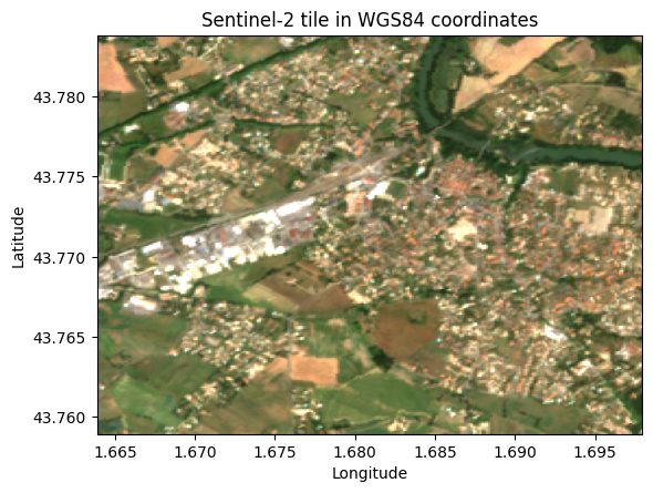

4.2 Interactive map with folium

For an interactive web map, use Folium to overlay the satellite image on a basemap:

import folium
from folium.raster_layers import ImageOverlay

center_lat = (south + north) / 2
center_lon = (west + east) / 2

m = folium.Map(location=[center_lat, center_lon], zoom_start=14)

ImageOverlay(
    image=rgb,
    bounds=[[south, west], [north, east]],
    opacity=0.7,
).add_to(m)

m

Make this Notebook Trusted to load map: File -> Trust Notebook

Exercise 8 — Display a Sentinel-2 tile on an interactive folium map

Goal: Reproject the tile bounds to WGS84 and display the RGB composite on an interactive folium map.

Steps:

Use transform_bounds() to convert the tile bounds from EPSG:3035 to EPSG:4326
Compute the centre of the tile (average of south/north and west/east)
Create a folium.Map centred on the tile
Add an ImageOverlay with the RGB array and WGS84 bounds

import folium
from folium.raster_layers import ImageOverlay
from rasterio.warp import transform_bounds

# Step 1: Reproject bounds to WGS84
west, south, east, north = ___  # TODO: transform_bounds(...)

# Step 2: Compute the centre
center_lat = ___  # TODO
center_lon = ___  # TODO

# Step 3: Create the folium map
m = ___  # TODO: folium.Map(...)

# Step 4: Add the satellite image overlay
___  # TODO: ImageOverlay(...).add_to(m)

m

Hint — Exercise 8

transform_bounds(tile_crs, "EPSG:4326", *tile_bounds) returns (west, south, east, north) in degrees.
Centre: center_lat = (south + north) / 2, center_lon = (west + east) / 2.
folium.Map(location=[center_lat, center_lon], zoom_start=14) creates the map.
ImageOverlay(image=rgb, bounds=[[south, west], [north, east]], opacity=0.7).add_to(m) overlays the image.

Solution — Exercise 8

import folium
from folium.raster_layers import ImageOverlay
from rasterio.warp import transform_bounds

west, south, east, north = transform_bounds(
    tile_crs, "EPSG:4326", *tile_bounds
)

center_lat = (south + north) / 2
center_lon = (west + east) / 2

m = folium.Map(location=[center_lat, center_lon], zoom_start=14)

ImageOverlay(
    image=rgb,
    bounds=[[south, west], [north, east]],
    opacity=0.7,
).add_to(m)

m

5 CLC+ Backbone Labels

CLC+ Backbone is a high-resolution land-cover product produced by the Copernicus Land Monitoring Service. It provides pixel-level land-cover classification across Europe at 10 m resolution, making it an ideal ground-truth dataset for training and evaluating segmentation models.

5.1 Land-cover classes

CLC+ Backbone uses 10 land-cover classes:

Class ID	Name	Description
1	Sealed	Buildings, roads, paved surfaces
2	Woody – needle leaved	Coniferous forests
3	Woody – broadleaved deciduous	Deciduous forests
4	Woody – broadleaved evergreen	Evergreen broadleaved forests
5	Low-growing woody plants	Bushes, shrubs
6	Permanent herbaceous	Grasslands, meadows
7	Periodically herbaceous	Croplands
8	Lichens and mosses	Natural low vegetation
9	Non- and sparsely-vegetated	Bare soil, rock
10	Water	Rivers, lakes, sea

5.2 Downloading labels

Labels can be downloaded through the Copernicus Land Monitoring Service REST API. The download_clcpluslabel() utility function handles this:

from utils import download_clcpluslabel, tiff_to_numpy

# Bounding box matching our FRJ27 tile (EPSG:3035)
bbox = [3649890, 2331750, 3652390, 2334250]

download_clcpluslabel("label_2018.tif", bbox, year=2018)
label_array = tiff_to_numpy("label_2018.tif")  # 2D array of class IDs (1-10)

The function queries the WCS endpoint of the CLC+ Backbone service, requesting the raster data for the specified bounding box and year.

5.3 Label–image alignment

The CLC+ labels and Sentinel-2 patches share the same CRS (EPSG:3035) and bounding box, which means they are spatially aligned by construction. Each pixel in the label corresponds to the same geographic area as the matching pixel in the satellite image.

Exercise 9 — Download a CLC+ label for a given tile and year

Goal: Download the CLC+ Backbone land-cover label that matches the FRJ27 Sentinel-2 patch and convert it to a NumPy array.

Steps:

Define the bounding box matching the FRJ27 tile (EPSG:3035): [3649890, 2331750, 3652390, 2334250]
Call download_clcpluslabel() with the filename, bounding box, and year
Convert the downloaded TIFF to a NumPy array using tiff_to_numpy()

from utils import download_clcpluslabel, tiff_to_numpy

# Bounding box matching the FRJ27 tile (EPSG:3035)
bbox = [3649890, 2331750, 3652390, 2334250]
year = 2018
filename = "test_label.tif"

# Step 1: Download the label
___  # TODO

# Step 2: Convert to NumPy array
img_array = ___  # TODO

Hint — Exercise 9

download_clcpluslabel(filename, bbox, year) downloads the label and saves it as a TIFF file.
tiff_to_numpy(filename) opens the TIFF, converts it to a NumPy array, cleans up nodata values (254, 255 → 0), and returns the array.

Solution — Exercise 9

from utils import download_clcpluslabel, tiff_to_numpy

bbox = [3649890, 2331750, 3652390, 2334250]
year = 2018
filename = "test_label.tif"

download_clcpluslabel(filename, bbox, year)
img_array = tiff_to_numpy(filename)

The training pipeline in section 2 expects labels as NumPy .npy files stored on S3, following a specific path convention. The expected S3 path structure is:

s3://projet-hackathon-ntts-2025/data-preprocessed/labels/CLCplus-Backbone/SENTINEL2/{NUTS}/{year}/{tile_size}/{patch_id}.npy

Exercise 10 — Save the label as .npy and upload to S3

Goal: Save the label array from Exercise 9 as a .npy file and upload it to S3 in the path expected by the training pipeline.

Steps:

Save img_array locally as a .npy file using np.save()
Initialise an S3FileSystem with get_file_system() (from utils, same as Exercise 2)
Build the S3 destination path matching the training pipeline convention
Upload the local file with fs.put()
Verify the upload by listing the S3 directory with fs.ls()

import numpy as np
from utils import get_file_system

# Step 1: Save the label array locally as .npy
local_path = "3649890_2331750_0_937.npy"
___  # TODO: np.save(local_path, img_array)

# Step 2: Initialise the S3 filesystem
fs = ___  # TODO: get_file_system()

# Step 3: Build the S3 destination path
s3_path = ___  # TODO: "projet-hackathon-ntts-2025/data-preprocessed/labels/CLCplus-Backbone/SENTINEL2/FRJ27/2018/250/3649890_2331750_0_937.npy"

# Step 4: Upload to S3
___  # TODO: fs.put(local_path, s3_path)

# Step 5: Verify the upload
print(fs.ls(___))  # TODO: S3 directory path (without filename)

Hint — Exercise 10

np.save("file.npy", array) saves a NumPy array to disk.
get_file_system() returns an s3fs.S3FileSystem configured with the SSP Cloud credentials.
The S3 path must not include the s3:// prefix when using fs.put() and fs.ls().
fs.put(local_path, s3_path) uploads a local file to S3.
fs.ls("projet-hackathon-ntts-2025/data-preprocessed/labels/CLCplus-Backbone/SENTINEL2/FRJ27/2018/250") lists all files in the directory.

Solution — Exercise 10

import numpy as np
from utils import get_file_system

local_path = "3649890_2331750_0_937.npy"
np.save(local_path, img_array)

fs = get_file_system()

s3_path = "projet-hackathon-ntts-2025/data-preprocessed/labels/CLCplus-Backbone/SENTINEL2/FRJ27/2018/250/3649890_2331750_0_937.npy"
fs.put(local_path, s3_path)

print(fs.ls("projet-hackathon-ntts-2025/data-preprocessed/labels/CLCplus-Backbone/SENTINEL2/FRJ27/2018/250"))

Exercise 11 — Plot the satellite image and CLC+ label side by side

Goal: Create a figure with two subplots: the Sentinel-2 RGB composite on the left and the CLC+ label map on the right, with a shared legend showing all 10 land-cover classes.

Steps:

Create a figure with plt.subplots(1, 2, ...)
Display the RGB array on the left subplot
Display the label array on the right subplot with the CLC+ colormap
Add a legend describing the 10 land-cover classes using Patch

import matplotlib.pyplot as plt
from matplotlib.colors import ListedColormap
from matplotlib.patches import Patch

# Classes & colormap (provided)
classes = [
    ("Sealed (1)", "#FF0100"),
    ("Woody -- needle leaved trees (2)", "#238B23"),
    ("Woody -- Broadleaved deciduous trees (3)", "#80FF00"),
    ("Woody -- Broadleaved evergreen trees (4)", "#00FF00"),
    ("Low-growing woody plants (bushes, shrubs) (5)", "#804000"),
    ("Permanent herbaceous (6)", "#CCF24E"),
    ("Periodically herbaceous (7)", "#FEFF80"),
    ("Lichens and mosses (8)", "#FF81FF"),
    ("Non- and sparsely-vegetated (9)", "#BFBFBF"),
    ("Water (10)", "#0080FF"),
]

cmap = ListedColormap([color for _, color in classes])

# Step 1: Create the figure
fig, axes = ___  # TODO: plt.subplots(1, 2, figsize=(12, 6))

# Step 2: Sentinel-2 RGB on the left
___  # TODO: axes[0].imshow(rgb)
___  # TODO: set title and turn off axis

# Step 3: CLC+ label on the right
___  # TODO: axes[1].imshow(img_array, cmap=cmap, vmin=1, vmax=10)
___  # TODO: set title and turn off axis

# Step 4: Legend
legend_elements = [
    ___  # TODO: Patch(facecolor=color, edgecolor="black", label=label)
    # for label, color in classes
]

fig.legend(
    handles=legend_elements,
    loc="center right",
    bbox_to_anchor=(1.35, 0.5),
    frameon=True,
)

plt.tight_layout()
plt.show()

Hint — Exercise 11

plt.subplots(1, 2, figsize=(12, 6)) returns a figure and an array of two axes.
Use axes[0].imshow(rgb) for the satellite image, and axes[1].imshow(img_array, cmap=cmap, vmin=1, vmax=10) for the label.
Turn off axes ticks with axes[i].axis("off").
Build the legend with a list comprehension: [Patch(facecolor=color, edgecolor="black", label=label) for label, color in classes].

Solution — Exercise 11

import matplotlib.pyplot as plt
from matplotlib.colors import ListedColormap
from matplotlib.patches import Patch

classes = [
    ("Sealed (1)", "#FF0100"),
    ("Woody -- needle leaved trees (2)", "#238B23"),
    ("Woody -- Broadleaved deciduous trees (3)", "#80FF00"),
    ("Woody -- Broadleaved evergreen trees (4)", "#00FF00"),
    ("Low-growing woody plants (bushes, shrubs) (5)", "#804000"),
    ("Permanent herbaceous (6)", "#CCF24E"),
    ("Periodically herbaceous (7)", "#FEFF80"),
    ("Lichens and mosses (8)", "#FF81FF"),
    ("Non- and sparsely-vegetated (9)", "#BFBFBF"),
    ("Water (10)", "#0080FF"),
]

cmap = ListedColormap([color for _, color in classes])

fig, axes = plt.subplots(1, 2, figsize=(12, 6))

axes[0].imshow(rgb)
axes[0].set_title("Sentinel-2 RGB")
axes[0].axis("off")

axes[1].imshow(img_array, cmap=cmap, vmin=1, vmax=10)
axes[1].set_title("CLC+ Label")
axes[1].axis("off")

legend_elements = [
    Patch(facecolor=color, edgecolor="black", label=label)
    for label, color in classes
]

fig.legend(
    handles=legend_elements,
    loc="center right",
    bbox_to_anchor=(1.35, 0.5),
    frameon=True,
)

plt.tight_layout()
plt.show()