This chapter covers the model lifecycle from an MLOps perspective. It is deliberately not about modelling choices — architecture, hyperparameter tuning, or loss functions are left to the practitioner — but about the operational scaffolding that makes a model trustworthy, reproducible, and maintainable in production. The four sections follow the natural order of the lifecycle: training reproducibly, validating beyond accuracy, packaging for deployment, and storing with versioning. Data management, the upstream step, is covered in the previous chapter.
Model training
Choosing the model, designing an appropriate Deep Learning architecture or applying best Machine Learning practices (preprocessing, cross-validation, dealing with class imbalance, parameter tuning…) falls outside the MLOps scope per se. Therefore, we will not cover these aspects here and instead refer to further references for details. From an MLOps perspective, what actually matters is being able to replicate the training in a fully reproducible way, at any time, on any machine that has sufficient computational power (e.g. GPU).
Once again, the idea is that if you lose everything - machine, storage…, you should be able to re-achieve your results without any additional effort.
This is achievable through different means and softwares, yet, minimally:
Fixed Randomness: random seed should be fixed for any process that implies randomness, including train/validation/test splitting, model training…
Version Control (Git) & Remote Repository hosting: the training code should be versioned using a version control system such as Git. The Git repository should be hosted on a remote source control management (SCM) platform (e.g., GitHub, a private GitLab instance, SCM-Manager, or similar). This ensures that the codebase is backed up, easily shared with other colleagues, and accessible independently of any local machine, which is essential for collaboration and traceability.
Modular Code: the training pipeline should be fully reproducible, as abstract as possible, with minimally hard-coded values and runnable with all sets of hyperparameters (and ideally for different models). Especially, avoid at all costs notebooks.
Experiment Tracking: there should be a logging tool (Tensorboard, MLflow, Weights & Biases…) for you to track experiments, metrics and hyperparameters (see below) including training code and data version.
Environment Definition: Define the exact execution environment (e.g., conda.yaml, requirements.txt, or a Docker image) to prevent “it works on my machine” failures.
Insee uses the library Hydra for seamless configuration management, enabling to have a very abstract and unified train.py script for every model architecture and hyperparameters,
uv for dependency management and environment definition,
torchTextClassifiers, an internally developed library that serves as a toolkit for text classification using deep learning and distributes a unified source of truth for the model design across training, inference… It is highly predicated on PyTorch and Lightning, with minimum other dependencies,
Argo Workflows is a Kubernetes-native software used to launch several parallel trainings in a fully reproducible way (on our Onyxia cluster),
and finally MLFlow is used as a logger and to monitor training.
Statistics Austria: reticulate in R for Keras and Tensorflow usage
To train our models, we use Keras and TensorFlow in R via reticulate to train our models. Retraining needs to be done on a quaterly basis, for each model. To ensure our outcome is reproducible and traceable, we implement the following standards.
Random seeds are used when splitting the data into training, test, and validation sets to ensure reproducibility. When new data becomes available, we generate a new split and store the corresponding observation IDs for each subset. By explicitly saving these IDs, we can always reconstruct the exact data used for training and evaluation of a given model. This makes it possible to trace and compare model results over time, even as the underlying dataset evolves.
We use Git for version control and host the code repositories on a private Bitbucket. With this, we enable collaborative coding and ensure that any changes to the project are traceable. Each modification is tracked through commits, allowing us to review the history of the project, identify when and why changes were made, and, if necessary, revert to earlier versions. In addition, we use branching and pull requests to manage parallel development, review contributions, and maintain code quality before integrating changes into the main codebase.
Since each model needs to be retrained quarterly, it is essential that our code is reproducible across multiple collaborators. To ensure consistency, we rely on a stable and well-documented training pipeline. Hyperparameter tuning is not performed at every retraining cycle; instead, we reuse the set of hyperparameters identified as optimal during the initial model development. These configurations are stored in YAML files, which makes them easy to reuse, track, and modify if adjustments become necessary. This approach reduces computational overhead while maintaining consistency in model performance across retraining cycles.
Training logs are stored for subsequent analysis. These logs are automatically generated by Keras during the training process and capture detailed information about the model’s performance at each epoch. In particular, they include metrics such as loss and accuracy over time, which allow us to monitor the learning progress and detect potential issues like overfitting or underfitting. In addition, the logs provide a record of overall model performance, enabling comparisons across different training runs and supporting reproducibility and model evaluation.
To avoid the problems of differing environments and package versions across collaborators, we use the renv package in R along with a project-specific lock file. This lock file (typically renv.lock) is a snapshot of the project’s R environment at a given point in time: it records the exact versions of all packages used, along with their sources and dependencies. When another collaborator opens the project, they can use this lock file to automatically reinstall those exact versions. This ensures that all dependencies (including exact package versions) are recorded and can be restored consistently, allowing every collaborator to run the code in an identical environment and hence reducing version-related issues.
German Federal Statistical Office: Spark-based text classification within Cloudera AI Workbench
At Destatis, these principles are implemented through a set of internal tools and platforms that ensure reproducibility, traceability, and collaboration across projects:
Code versioning and repository hosting: our codebases are versioned using Git and hosted on internal source control platforms, either a private instance of GitLab or SCM-Manager. These platforms provide centralized repositories, access control, and collaboration features (e.g., merge requests and code reviews), while ensuring that all code is securely stored and backed up within the organization.
Experiment tracking: we use MLFlow as our main experiment tracking tool in both of our development environments (R-Server and Cloudera). MLflow allows us to log experiments, including metrics, hyperparameters, artifacts, and the associated code version, ensuring that every training run can be reproduced and compared with previous experiments.
Pipeline development on Cloudera: when developing pipelines within the Cloudera environment, we rely on the Cloudera AI Workbench framework provided by Cloudera. This framework builds on MLflow and integrates experiment tracking, model management, and execution into a unified, user-friendly interface, which simplifies the development and monitoring of machine learning workflows on the platform. In practice, Cloudera AI provides many convenient features and a more user-friendly, low-code interface, which can be a useful compromise for teams with heterogeneous technical profiles. However, it may also create a certain lock-in effect; since the framework ultimately builds on the open-source MLflow ecosystem, investing time in learning MLflow directly can provide greater flexibility and independence in the long run.
Focus: Model training at scale with Spark - general lessons learned
When text classification datasets grow beyond the limits of single-machine parallelization in Python or R, distributed frameworks such as Apache Spark become a natural consideration. Spark enables horizontal scaling across clusters and is particularly well suited for large-scale data preparation, feature extraction, and the training of classical machine-learning models on datasets that no longer fit into memory. In an MLOps context, Spark integrates well with cloud storage, columnar formats such as Parquet, and fault-tolerant execution, making it attractive for industrial and institutional environments.
However, experience shows that Spark should be used selectively for model training. While it excels at scaling data processing and simple models, its native machine-learning library (MLlib) offers a limited algorithm portfolio and constrained options for hyperparameter tuning and model optimization. As a result, Spark-based ML pipelines are most effective when applied to well-understood, classical models and when training speed, robustness, and operational scalability are prioritized over modeling flexibility. For modern NLP approaches—particularly those based on transformer architectures—Spark is typically better positioned as a data engineering backbone rather than as the primary training framework.
These general observations are confirmed by practical experience at Destatis, where Spark was evaluated for large-scale text-to-code classification in the context of COICOP expenditure coding. Several experiments were conducted on both a traditional R-based infrastructure and a Cloudera Spark environment, focusing on performance, scalability, and operational feasibility.
The results show that classical models can achieve solid predictive performance across platforms. A Random Forest model trained on an R server delivered strong results (Macro F1 ≈ 0.80, Accuracy ≈ 0.90) but required very high memory consumption (~200 GB) and its hyperparameters could only be fine-tuned on data subsamples, limiting its suitability for regular re-trainings. Logistic regression experiments on the R server using scikit-learn failed to converge or required runtimes that were considered too risky for production use.
In contrast, logistic regression implemented with Spark MLlib achieved competitive performance (Macro F1 ≈ 0.78, Accuracy ≈ 0.88) while dramatically reducing training time (3–5 minutes) and keeping memory usage at a manageable level (~40 GB). Even with grid search over multiple parameter combinations, total runtimes remained operationally acceptable. More complex models, such as Random Forests in MLlib, proved unsuitable for this high-cardinality multi-class problem, leading to memory errors and limited model quality.
Overall, this experience illustrates a key MLOps takeaway: Spark can be highly effective for scalable, robust training of classical text classification models, especially when retraining frequency, runtime stability, and infrastructure constraints matter. At the same time, its limitations in model diversity and optimization flexibility mean that Spark-based ML should be carefully scoped, especially in text classification context.
Model validation
MLOps induces a notion of operations, meaning that your model will be served and deployed for a specific - potentially critical - use-case, and used by production teams.
Therefore, you need to ensure your model is trustworthy and will not break the production pipeline via a meaningful set of metrics on top of mere accuracy.
The choice of these metrics strongly depends on the use case and the design of the production pipeline. In a text-to-code context, evaluation must account for the specific characteristics of statistical classification systems: a large number of classes, strong class imbalance, and high semantic proximity between categories. These challenges have several implications for evaluation:
Overall accuracy alone is rarely sufficient and may even be misleading. Instead, evaluation strategies should emphasize precision, recall, and F1-score, which provide a more meaningful view of model behavior under imbalance.
In multi-class settings like here, the aggregation strategy of metrics is a critical design choice. Macro, micro, and weighted variants of F1-score answer different questions and should be selected based on how classification errors are valued. If errors on small or rare classes are substantively important, unweighted macro metrics are preferable, as they prevent dominant classes from masking poor performance elsewhere. Conversely, weighted metrics may be appropriate when the operational focus is primarily on high-frequency categories. In all cases, relying solely on aggregated metrics is insufficient; class-level evaluation is essential to identify systematic biases and uneven model performance.
Evaluation datasets should be constructed carefully to ensure representativeness. Stratified train–test splits by class are generally recommended, as they help preserve the distribution of both frequent and rare categories and enable more reliable performance estimates across classes.
Finally, evaluation datasets must be representative of future data, not just historical samples. Regular evaluation on newly collected data, combined with expert review, is necessary to detect model drift and to ensure sustainable model quality over time.
In many automatic coding use cases, low-confidence predictions are routed to human experts. In this context, model confidence scores must be well calibrated — that is, they should reflect true probabilities (e.g., a confidence of 0.9 should correspond to a 90% probability of being correct): this is called calibration (see Understanding Model Calibration for further reading). Hardware-specific metrics like latency (how fast is the inference?) and memory footprint are also common.
ImportantThe Gold Standard in MLOps
An automated validation script that runs immediately after training, compares results against a baseline (the current “Champion” model), and logs the report alongside the model artifact.
Insee: Calibration is key
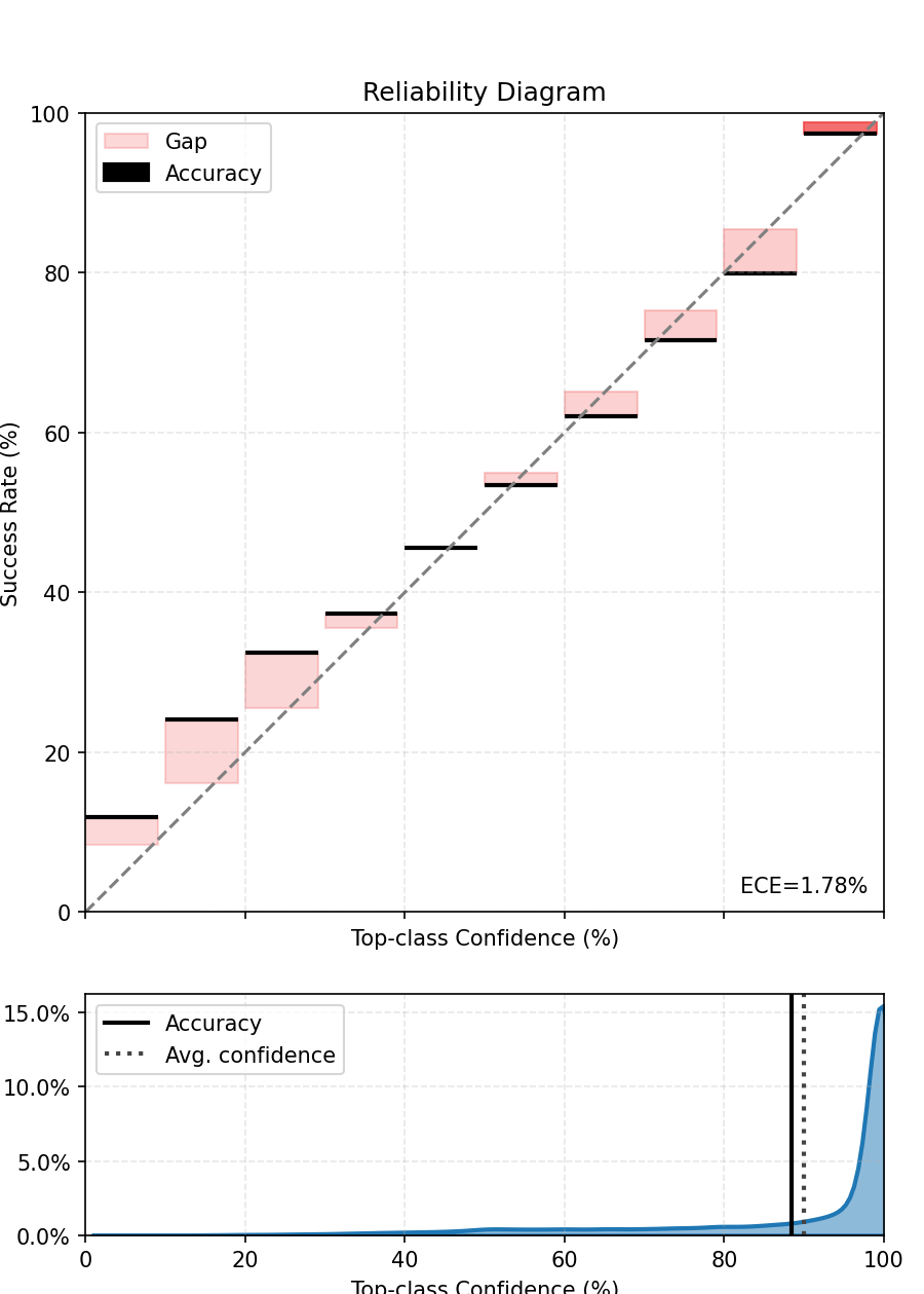
For the NACE coding pipeline at Insee, the model does not operate in isolation: when its confidence score falls below a defined threshold, the prediction is discarded and the observation is routed to a human annotator (human-in-the-loop). This design places a strong requirement on the model beyond raw accuracy — its confidence scores must be calibrated, meaning that they should reflect true probabilities. Concretely, among all predictions assigned a confidence of 0.8, approximately 80% should indeed be correct.
Measuring calibration: the Expected Calibration Error (ECE)
The Expected Calibration Error (ECE) is the standard scalar metric for quantifying miscalibration. It is computed by bucketing predictions into confidence bins and measuring, for each bin, the gap between the average confidence and the observed accuracy:
where \(B_b\) is the set of samples in bin \(b\), \(n\) is the total number of samples, \(\text{acc}(B_b)\) is the fraction of correct predictions in that bin, and \(\text{conf}(B_b)\) is the mean confidence. A perfectly calibrated model yields ECE = 0; in practice, values below 0.05 are generally considered acceptable.
Visualising calibration: the reliability diagram
The reliability diagram (or calibration curve) provides a visual counterpart to the ECE. Each point plots the mean confidence of a bin against its observed accuracy. A perfectly calibrated model lies on the diagonal; points above indicate overconfidence, points below indicate underconfidence.
Reliability diagram computed on the validation set, using the torch-uncertainty library
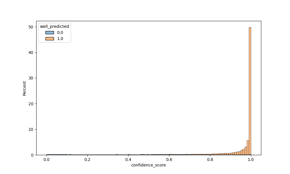
Visualising separation: the confidence distribution
A complementary diagnostic is the confidence distribution stratified by prediction correctness. Ideally, correct predictions cluster near high confidence values and incorrect predictions near low ones — indicating that the model’s uncertainty is a reliable signal for the human-in-the-loop routing decision.
Confidence distribution stratified by prediction correctness
Statistics Austria: Automated model evaluation
Before the model is deployed, several validation steps are performed. These include the calculation of evaluation metrics and a comparison with the previous model version. Evaluation metrics are automatically generated each time the model is retrained. Metrics such as accuracy, F1 score, and top-k accuracy are then compared against those of earlier model versions.
In addition, since ground-truth labels are not immediately available for new data, we perform a consistency check against the previous model’s predictions. A dedicated script compares the newly predicted class labels with those from the earlier model, for example by examining the distribution of predicted classes. This allows us to detect unexpected shifts or anomalies in the model’s behavior and provides an additional safeguard before deployment.
We also pay particular attention to model performance on underrepresented classes. To this end, we compare macro- and micro-averaged F1 scores: while micro F1 reflects overall performance weighted by class frequency, macro F1 gives equal weight to each class and therefore highlights potential weaknesses on rare classes. This helps ensure that improvements in aggregate performance do not come at the expense of minority classes.
German Federal Statistical Office: evaluation strategy for the specific Text-To-Code context
These principles were applied in practice at Destatis in the context of large-scale COICOP text-to-code classification. Given the highly imbalanced class distribution and the presence of several hundred target classes, the evaluation strategy deliberately moved beyond accuracy as a primary metric. While accuracy was still reported, the main focus was placed on precision, recall, and F1-score, which better capture performance differences across classes of varying frequency.
In particular, unweighted macro F1-score was chosen as a key benchmark metric. This choice reflects the statistical objective of treating all COICOP categories as equally important, regardless of their frequency in the data, and of avoiding systematic neglect of rare but substantively relevant classes. Weighted metrics were considered but deemed less suitable, as they tend to understate errors on small classes and can mask biased prediction patterns—for example, consistently favoring dominant categories over closely related but less frequent ones.
To support robust evaluation, all train–test splits were stratified by COICOP class, ensuring that both frequent and rare categories were adequately represented in the test data. In addition to aggregated metrics, class-level performance indicators were systematically analyzed to identify weak classes and guide targeted improvements, such as enriching training data for problematic categories.
Finally, evaluation at Destatis extended beyond static test sets. To measure the robustness of the different models and to ensure relevance for future production use, model outputs were compared with classifications produced by domain experts. This concerns records where the model scores used in production were below a fixed thresholds. This continuous expert-based validation targeting difficult records ensures that the model remains aligned with evolving data and classification practices and naturally forms the basis for a human-in-the-loop framework, which will be discussed in the following sections.
Model wrapping
Any machine learning model would expect a nicely preprocessed (or tokenized) tensors as input, and outputs logits (or confidence scores).
Yet in production, we have to take a step back: the user directly inputs raw text into the pipeline, and expects a label back.
The wrapper is the object that bridges the gap between machine learning and ops, and is the object that will be actually deployed. It encapsulates the trained model and handles:
Preprocessing: All cleaning, normalization, and tokenization steps.
Inference: Passing the data through the model.
Post-processing: Converting raw logits into human-readable predictions or nomenclature codes.
Standardizing this into a single .predict() method allows the production team to swap models without changing a single line of their application code.
Many libraries, for instance MLFlow or Lightning, provide native support for these wrapper objects.
Insee: MLflow integration with a PyTorch model
The in-house library torchTextClassifiers (TTC) provides an end-to-end interface from raw text to predicted labels, encapsulating tokenisation, model inference, and confidence scoring. It exposes a PyTorch Lightning module, which integrates natively with the MLflow Logger to automatically record metrics, hyperparameters, and checkpoints during training — with no boilerplate.
Serving the model as an MLflow pyfunc
MLflow’s custom pyfunc flavour provides a framework-agnostic interface for model serving: once logged, the model can be loaded and called uniformly regardless of the underlying framework, and deployed to any MLflow-compatible serving infrastructure.
The wrapper below packages a trained TTC object as a pyfunc model. At inference time, it expects a DataFrame whose first column contains the raw text to classify (additional columns can carry categorical features). It returns the predicted label together with its associated confidence score.
At serving time, the model is loaded with mlflow.pyfunc.load_model(...) and called via its .predict() method, making it transparent to the downstream inference pipeline.
Statistics Austria: Wrapping up pre- and postprocessing
We implemented a wrapper around the trained model in the form of a single function that handles all pre- and post-processing steps required for inference. This function serves as the interface between raw user input and the model, ensuring that the full prediction pipeline is standardized and reproducible.
During pre-processing, raw input data is transformed into a format suitable for the model. In particular, text inputs are tokenized, and categorical variables—often provided in textual form—are mapped to the corresponding integer encodings used internally by the model.
During inference, the processed inputs are passed through the trained model, which outputs a vector of probabilities, with one value for each possible class or code.
During post-processing, these outputs are converted into user-friendly predictions. Specifically, the probabilities are sorted to generate the top-k most likely codes for each input.
By encapsulating all these steps in a single .predict() function, we create a clear and stable interface for deployment. This allows the underlying model to be updated or replaced without requiring changes to the surrounding application code, effectively decoupling machine learning development from production systems.
German Federal Statistical Office: model wrapping with Cloudera AI Workbench
Cloudera AI Workbench provides an easy to use functionality that allows to deploy machine learning models efficiently. Using Cloudera AI, it is possible to deploy automated pipelines for analytics workloads in different programming languages such as R or Python. In addition, you can train, evaluate and deploy models as REST APIs that serve predictions to other applications or services. Predictions can be easily generated through a user-defined function, which returns the results in JSON format. This allows to efficiently integrate the model outputs into external systems and workflows.
The following code shows a simple example of a basic function. This function can be used within a deployment setup to return outputs in JSON format.
Code
import pickleimport numpy as np# load model# with open("model.pkl", "rb") as f:# model = pickle.load(f) # with open("labels.pkl", "rb") as f:# labels = pickle.load(f) def predict(args): data = args["input"] features = np.array(data["features"]).reshape(1, -1) pred = model.predict(features)[0] species = labels[pred]return {"prediction_index": int(pred),"prediction_label": species }
In Cloudera Machine Learning, a model is built around a script that usually contains a function. This function takes input data in JSON format, processes it using the model logic, and returns results in JASON format. The model itself consists of two main parts: the implementation and the trained parameters. These are combined during the build stage, where the system packages everything into a fixed, versioned artifact called a model build. Each build is static and immutable, so any changes require creating a new version. During this build process, CML creates a Docker-based environment and installs any required dependencies. In the deployment stage, this build is turned into a running service with defined resources (CPU, memory) and possibly multiple replicas to handle parallel requests. Each replica processes one request at a time, so having several improves performance and reliability. Once deployed, the model is accessible via a REST API. Due to the simplified deployment, the model functionality in Cloudera AI is straightforward and easy to use. However, its simplicity limits flexibility. For example, there are fewer built-in options for experiment tracking, advanced model diagnostics and less flexibility in custom deployment pipelines.
Model storage & versioning
Exactly as for data, and for the same reasons, models should be stored in a stable storage, once again preferably cloud-based, called the Model Registry. The logger you (should) have used for training most of the time also handles the storage of them.
A standard practice is also to keep track of which model has been deployed over the time (versioning) via a promotion system: the registry acts as a “source of truth” for which model is currently in production.
The deployed model is treated exactly as a software application: it is versioned, tagged, updated/deprecated over time.
The rationale is that you should be able to load any experiment that you have tried, at any time. This system ensures that the production pipeline is model-agnostic; the application simply fetches the model tagged as Production, regardless of whether it is an SVM or a Transformer.
Insee: Model storage and versioning with MLflow
At Insee, MLflow serves as the single source of truth for both training monitoring and model storage, covering the full lifecycle from experiment to production.
Experiment tracking. During training, metrics and hyperparameters are logged in real time to an MLflow experiment — a named collection of runs. Each run records the full training context (loss curves, validation scores, parameters, code version), making any past experiment reproducible and comparable at a glance.
Model logging. At the end of a run, the trained model is logged as an artifact using the pyfunc wrapper described above. This decouples the model artefact from the framework used to train it and ensures it can be loaded and served uniformly.
Model registry and promotion. Once a run is deemed satisfactory, its model artifact is registered in the MLflow Model Registry under a versioned name. Versions progress through explicit lifecycle stages — Staging, then Production — via a promotion step that requires a deliberate human decision. The production pipeline always fetches the model tagged Production, remaining entirely agnostic to the underlying architecture.
This workflow ensures that rolling back to a previous version is as simple as changing a tag, and that every model ever trained can be reloaded from its run ID at any point in time.
Statistics Austria: Switching model versions on RSConnect
Model versions are stored in a structured and versioned manner in stable storage. Each time a model is (re-)trained, all relevant artifacts are saved, including the trained model itself, hyperparameters, tokenizers, translation tables, and the corresponding version of the R code used for training, evaluation, and serving.
This setup acts as our “model registry”, allowing us to keep track of different model versions over time. Once deployed to the rsconnect server, we can switch between these versions, enabling the reproduction of past experiments and consistent rollback if needed.
By treating models as versioned artifacts, we ensure that any previously trained model can be reloaded and used at a later point. This makes the production pipeline largely model-agnostic, as the application can serve whichever model version is currently designated for deployment without requiring changes to the surrounding code.
German Federal Statistical Office: model storage & versioning
Cloudera AI offers a model registry for model tracking and management of their lifecycle. This also enables users to roll back to previous model versions if necessary. Similar to model wrapping, the model storage process is simplified, making it easier to store, organize, and deploy models. The model registry is built on MLFlow, much like the component used for tracking model experiments.
MLFlow is also the primary tool in our other development environment (R-Server), where it is used directly, without the interface provided by Cloudera.