Monitoring
Shipping a model is not the end of the MLOps lifecycle — it is the point where a new class of risks appears. In production, a model is exposed to inputs it never saw during training, to a real world that keeps drifting away from the training distribution, and, for classification tasks, to nomenclatures whose definitions can themselves change over time. None of these failures crash the API: predictions keep flowing, they just slowly get worse, unless something is actively watching.
Two practices close this gap:
- Observability: continuously assess whether current predictions can still be trusted. This combines label-free signals (e.g. comparing successive model versions, tracking known hard cases) with label-based ones (accuracy, calibration) whenever ground truth is available, complemented by human review where automation cannot cover everything.
- Retraining: turn newly collected and freshly labelled data into a reproducible pipeline that regularly produces a new, validated model version — closing the loop between what monitoring detects and what gets fixed.
Observability and retraining are two sides of the same loop: what monitoring flags becomes the training signal for the next model version.
Observability
Insee: GRAAL — an agentic approach to monitoring and relabelling
Beyond the automated reports described below, the production NACE coding pipeline (see the Data, Model and Serving chapters) is also watched continuously by human annotators reviewing a sample of live predictions — a signal that complements automated metrics and feeds back into retraining.
That level of continuous annotation isn’t sustainable for every pipeline, though, and nomenclatures are periodically revised, forcing costly relabelling of historical data. GRAAL (Graph-based Research with Agents for Automatic Labelling) is an Insee framework exploring an LLM-based answer to these gaps, for classifiers running fully offline on CPU whose reference knowledge is a set of official notices. An initial zero-shot RAG attempt — embedding notices and company declarations to retrieve the closest match — struggled because short, informal declarations and long, formal notices don’t share a comparable embedding space. GRAAL has since moved to a graph-exploring multi-agent system instead: nomenclature notices are modelled as a tree in a Neo4j database, and agents navigate it with dedicated tools (fetch a code’s definition, list children or siblings…) rather than similarity search, producing an explicit justification for every decision instead of an opaque distance score. Today GRAAL is used for monitoring existing API predictions, batch (re)coding on nomenclature changes, and generating synthetic training data — see the full presentation here.
Statistics Austria: Monitoring Reports
After each retraining phase, two quality reports are generated to monitor model performance and ensure consistency over time.
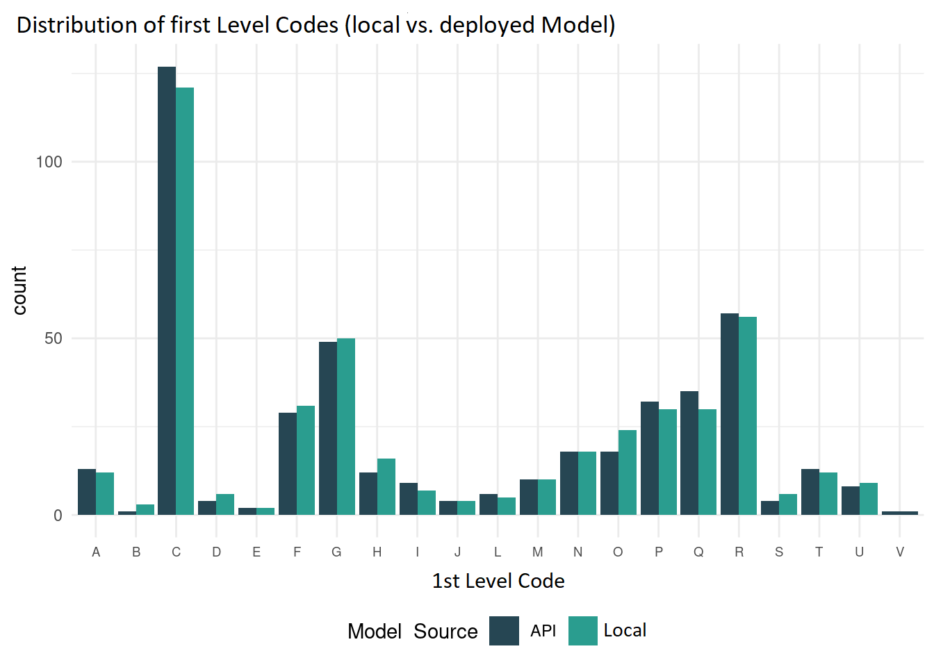
The first report focuses on comparing two model versions, typically the most recent model and its predecessor. Since true labels are not required for this comparison, the analysis is based on the models’ predictions. Predictions from both models are collected using the same data inputs. We compute and visualize the overall agreement rate between the models, as well as the distribution of predicted 1-digit codes. In addition, we evaluate a selected set of input texts that are known to be challenging in manual coding. For these cases, we analyze how both model versions classify them and compare the predictions to human annotations. This provides a qualitative assessment of behavioral changes between model versions.
The second report is based on the labeled validation data and therefore allows for a more formal performance evaluation. Standard metrics such as accuracy, top-k accuracy, and F1 score are calculated and visualized. This enables a quantitative assessment of model performance and facilitates comparisons across retraining cycles.
Below are examples of plots inclueded in the quality reports. A simple visualization of predicted first digits codes of the model currently in production, and the newly retrained model helps identify large prediction shifts easily. Severe differences in predictions on the first level may indicate that the newly trained model has learned substantially different patterns or behaves differently from the previous model, and therefore call for further inspection.
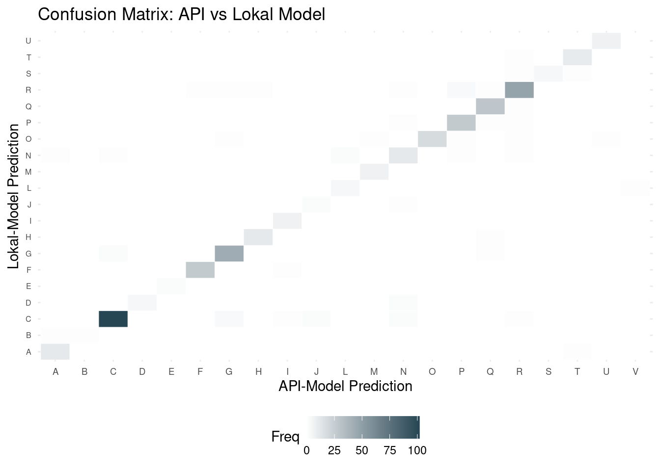
For a more detailed comparison of the predictions made by the model currently in production (API model) and the newly retrained local model, confusion matrices can be used. The diagonal represents cases where both models assigned the same first-digit code, while off-diagonal cells indicate disagreements between the two models. A strong concentration of observations along the diagonal therefore suggests a high level of agreement. More pronounced off-diagonal cells, such as the difference observed between the predictions of the two models for code C and G, indicate prediction shifts that may require further inspection.
German Federal Statistical Office: Dashboard & HITL (human-in-the-loop)
To ensure a smooth operation and reliability of the machine learning classification system, comprehensive observability measures were implemented. First of all, these include a dashboard that displays up to date operational data. This data is used for key visualizations to track the daily number of labels assigned by the machine learning algortihm, as well as the proportions of different labels assigned each day. Additionally, domain-specific metrics such as the average number and amount of expenses, and the categories used by participating households, are plotted to provide more detailed insights for the domain experts. Deviations in these metrics serve as indicators of anomalies. This proactive monitoring allows to quickly identify and address issues.
Furthermore, a human-in-the-loop approach is integrated where the collected data and the corresponding classifications are reviewed by domain experts. This manual review process ensures that any classification errors are promptly identified and corrected. Large correction lists are maintained to document these errors and facilitate continuous improvement of the system.
In cases where systematic errors with significant impact are detected, we prioritize the retraining of the machine learning algorithm to address these issues and enhance the overall accuracy and reliability of the classification system. This combination of automated monitoring and human oversight ensures robust observability and maintains the integrity of our data classification processes.
Retraining
Insee: Retraining stays classic
Retraining itself follows the same standard, reproducible pipeline described in chapter 2: fixed random seeds, versioned train/test/validation splits, and a tracked execution environment. What GRAAL changes is only what happens upstream of it — its batch recoding and synthetic-data generation are used to refresh the labelled dataset when a nomenclature changes version or annotation coverage is too thin, before handing off to that same classic retraining pipeline.
Statistics Austria: Reproducible retraining pipelines
The models are retrained on a quarterly basis as new training data becomes available. During each retraining cycle, the newly collected data is first fetched and combined with the existing historical training dataset to ensure that the model benefits from both recent and previously observed examples.
Based on the updated dataset, new training, test, and validation splits are created using predefined random seeds to ensure reproducibility. The observation IDs belonging to each split are stored so that the exact data partition used for a given model version can always be reconstructed and traced.
The retraining itself follows a standardized and reproducible pipeline, including the reuse of the established hyperparameter configuration and preprocessing steps.
After retraining, the two quality reports, described in section Observability, are generated. Together, they provide both label-free and label-based evaluations, ensuring that changes in model behavior are detected even when ground-truth data is limited or delayed.
German Federal Statistical Office: Retraining pipeline
Retraining of the model takes place approximately every two months to make sure there is no significant data drift. However, as mentioned, if significant errors are known, retraining is done immediately. An ongoing process involves experts providing corrections and feedback through regular testing of the classification systems, resulting in manual correction lists for the training data. These correction lists are applied to both old and new data. If systematic errors are discovered in the data sources, these are corrected through adjustments in the preprocessing step or the affected data is excluded.
Within the training pipeline, the data is initially split into training and test data in an 80/20 ratio with a fixed random seed. This is followed by hyperparameter tuning through repeated training runs to determine the best parameters. The selection of the best model is based on accuracy and the F1-score compared to the old model. Finally, a sanity test is conducted to check the entire classification system, including the model in the implemented application code as well as preprocessing and postprocessing, using prepared test cases. These test cases include, for example, common errors or added corrections.