# Models
EMB_MODEL_NAME = "qwen3-embedding-8b" # Embedding model
GEN_MODEL_NAME = "gemma4-26b-moe" # Generative model
# Qdrant
COLLECTION_NAME = "nace-collection"
RETRIEVER_LIMIT = 5 # Number of candidates returned by the vector search
# Generation
TEMPERATURE = 0.1 # Low temperature → more deterministic, reproducible outputs
# Evaluation
SAMPLE_SIZE = 100 # Number of activities to evaluate (increase for more robust results)RAG pipeline approach - Query a LLM for automatic coding
Forewords
This second RAG tutorial builds on the vector database created in part 1. It completes the RAG pipeline by loading labelled data, retrieving context from Qdrant, and generating final answers from a query. You will learn how to automatically classify free-text activity labels into the NACE 2.1 nomenclature, and then evaluate the quality of the pipeline at each stage.
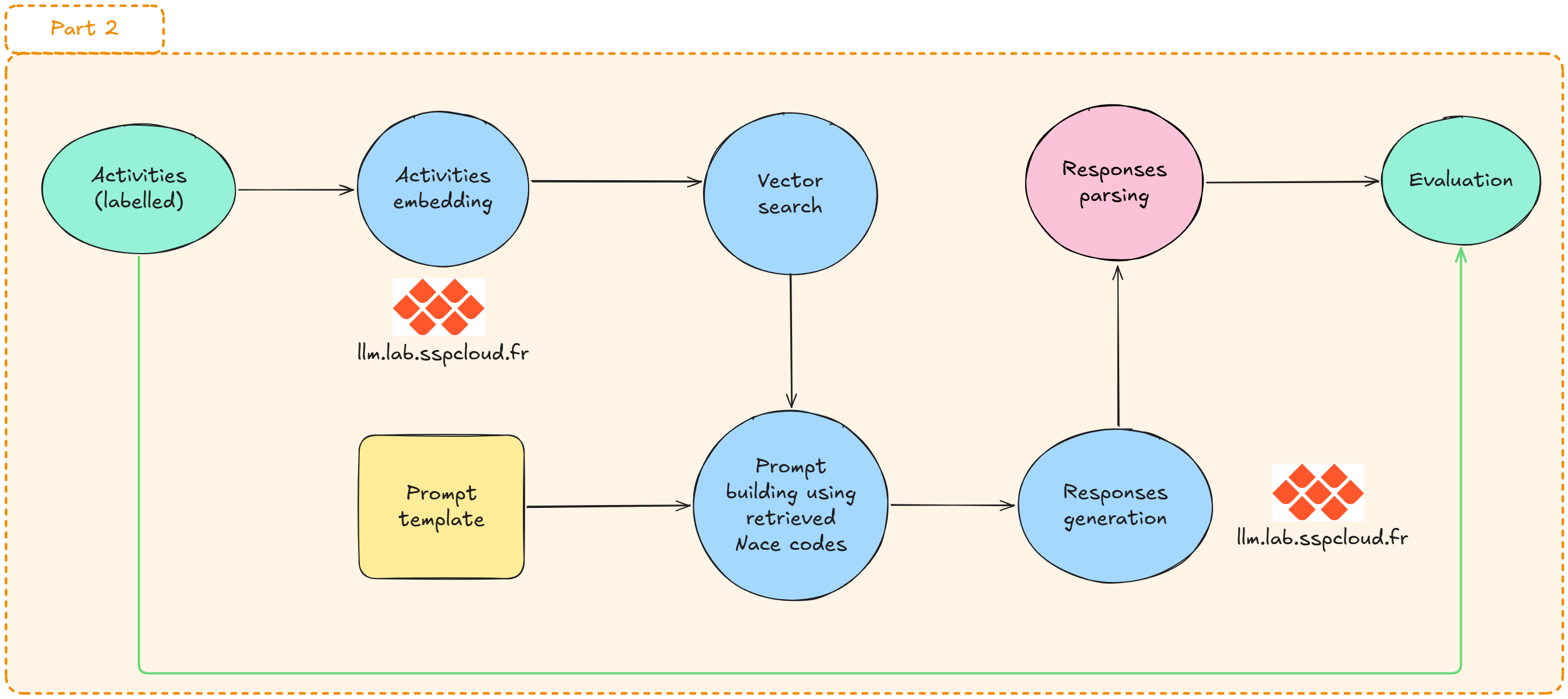
RAG pipeline overview
The automated coding workflow is broken down into five steps:
Raw text label
      │
      ▼
 [1] Embedding       ← transform the label into a dense vector
      │
      ▼
 [2] Retrieval       ← find the k nearest neighbours in Qdrant
      │
      ▼
 [3] Augmentation    ← inject retrieved candidates into a structured prompt
      │
      ▼
 [4] Generation      ← LLM inference with a JSON-constrained output
      │
      ▼
 [5] Evaluation      ← compare predictions against reference codes
The RAG acronym specifically refers to the combination of steps 2 (Retrieval) and 4 (Generation): instead of asking the LLM to code from memory — which would be unreliable for fine-grained nomenclatures — we supply it with the most semantically relevant candidates from the vector store.
Why do we need the generation step?
Retrieval gives us the top-k most semantically similar NACE descriptions for a given activity label — but it doesn’t pick the right code. For our use case, the generation step is what turns a list of candidates into a single classification decision:
- Disambiguation among close candidates: the top-5 retrieved codes often look very similar (e.g. several variants of “retail trade”). The LLM compares them against the full activity label and chooses the most specific one.
- Handling imprecise or messy inputs: real activity labels are often short, abbreviated or ambiguous. The LLM can interpret them by leveraging the retrieved definitions as context.
- Structured output: by constraining the LLM to return a JSON with the chosen NACE code, we get a directly usable prediction — not free-form prose.
In this notebook, you will:
- Load and inspect annotated examples
- Connect to Qdrant and check available collections
- Build a retrieval + generation function that queries Qdrant and sends retrieved context to an LLM
- Compare predicted labels with ground truth for evaluation
- Understand how retrieval quality affects final generation quality
Prerequisites
- Completion of tutorial 1 (creation of the
nace-collectionQdrant collection) - Access to the following services: LLM Lab, Qdrant
- Python libraries:
openai,qdrant-client,duckdb,pandas,tqdm,matplotlib
Connections and global parameters
Note
Why a low temperature? Temperature controls the degree of randomness in generation. For a closed-list classification task, we want stable and reproducible answers: a value between 0.0 and 0.2 is recommended. Higher values are better suited to creative tasks.
First attempt on a single activity label
Before running the pipeline on the full dataset, test each component step by step.
The following questions will follow the steps described below.
Inference on multiple activities
Next, let’s use some synthetic data. We will:
- run automatic classification on a sample of labelled activities,
- build metrics to evaluate the quality of the coding process.
Load the data
import duckdb

con = duckdb.connect(database=":memory:")

con.execute("INSTALL httpfs;")
con.execute("LOAD httpfs;")

query_definition = f"""
SELECT *
FROM read_parquet(
  'https://minio.lab.sspcloud.fr/projet-formation/diffusion/funathon/2026/project2/generation_None_temp08.parquet'
)
USING SAMPLE {SAMPLE_SIZE}
"""

annotations = (
    con.sql(query_definition)
    .to_df()
    .to_dict(orient="records")
)
print(f"Dataset loaded: {len(annotations)} rows")
print(f"Keys: {list(annotations[0].keys())}")
annotations[:2]
Dataset loaded: 100 rows
Keys: ['code', 'name', 'label'][{'code': '70.20',
'name': 'Business and other management consultancy activities',
'label': 'Budgeting and forecasting methodology design'},
{'code': '01.11',
'name': 'Growing of cereals, other than rice, leguminous crops and oil seeds',
'label': 'Soya bean farming and related operations'}]
Note
Dataset structure: Each row contains a free-text activity label (activity) and its reference NACE 2.1 code (nace_code). These annotations were generated by an agentic AI system and constitute synthetic data. As such, they are well-suited for testing a RAG pipeline on English-language activity labels, but no claim is made about whether they are representative of real-world annotation data.
Utility function: a full pipeline call
Before looping, we encapsulate steps 1–4 into a reusable function.
def run_rag_pipeline(activity: str) -> dict:
    """
    Run the full RAG pipeline for a single activity label.

    Parameters
    ----------
    activity : str
        Free-text economic activity label to be coded.

    Returns
    -------
    dict with keys:
        - nace_code (str | None) : predicted NACE code
        - codable (bool)        : True if the label could be coded
        - confidence (float)    : confidence score (0–1)
        - retrieved_codes (list): candidates returned by the retriever
    """
    # --- Step 1: Embedding ---
    emb_response = client_llmlab.embeddings.create(model=EMB_MODEL_NAME, input=activity)
    embedding = emb_response.data[0].embedding

    # --- Step 2: Retrieval ---
    points = client_qdrant.query_points(
        collection_name=COLLECTION_NAME,
        query=embedding,
        limit=RETRIEVER_LIMIT,
    )
    descriptions_retrieved = []
    codes_retrieved = []
    for point in points.model_dump()["points"]:
        descriptions_retrieved.append(point["payload"]["text"])
        codes_retrieved.append(point["payload"]["code"])

    # --- Step 3: Prompt construction ---
    user_prompt = USER_PROMPT_TEMPLATE.format(
        activity=activity,
        proposed_nace_descriptions="## " + "\n\n## ".join(descriptions_retrieved),
        proposed_nace_codes=", ".join(codes_retrieved),
    )

    # --- Step 4: LLM inference ---
    gen_response = client_llmlab.chat.completions.parse(
        model=GEN_MODEL_NAME,
        messages=[
            {"role": "system", "content": SYSTEM_PROMPT},
            {"role": "user", "content": user_prompt},
        ],
        temperature=TEMPERATURE,
        response_format=NaceClassificationResult,
    )

    result = gen_response.choices[0].message.parsed.model_dump()
    # Keep retrieved candidates for retriever evaluation
    result["retrieved_codes"] = codes_retrieved

    return result
Inference loop
Pipeline evaluation
To understand where the pipeline succeeds or fails, we evaluate each stage separately. Three metrics are useful here.
              ┌─────────────────────────────────────────────────┐
              │             EVALUATION METRICS                  │
              ├──────────────────┬──────────────────────────────┤
              │ Retriever@k      │ Is the correct code among    │
              │ accuracy         │ the k retrieved candidates?  │
              ├──────────────────┼──────────────────────────────┤
              │ LLM accuracy     │ When the retriever succeeded,│
              │ (conditional)    │ does the LLM pick the right  │
              │                  │ code?                        │
              ├──────────────────┼──────────────────────────────┤
              │ Pipeline         │ Is the final predicted code  │
              │ accuracy         │ correct? (end-to-end)        │
              └──────────────────┴──────────────────────────────┘
These three metrics are related by:
\[\text{Pipeline accuracy} = \text{Retriever@k} \times \text{LLM accuracy (conditional)}\]
This decomposition helps pinpoint whether errors come from the retriever or the LLM, and guides improvement efforts.
Tip Exercise 3: Compute evaluation metrics
Prepare evaluation columns
Before computing any metric, add three boolean columns to results:
retriever_hit: whether the true NACE code is among thekcandidates returned by Qdrantpipeline_correct: whether the predicted code matches the true codellm_correct_given_retriever: same aspipeline_correct, but set toNonewhen the retriever did not return the true code
Click to see the answer
# Is the true code among the retriever's candidates?
results["retriever_hit"] = results.apply(
    lambda row: row["true_code"] in row["retrieved_codes"], axis=1
)

# Is the predicted code correct?
results["pipeline_correct"] = results["pred_code"] == results["true_code"]

# Did the LLM pick the right code, given that the retriever found it?
results["llm_correct_given_retriever"] = results.apply(
    lambda row: row["pipeline_correct"] if row["retriever_hit"] else None,
    axis=1
)| activity | true_code | pred_code | retriever_hit | pipeline_correct | llm_correct_given_retriever | |
|---|---|---|---|---|---|---|
| 0 | Budgeting and forecasting methodology design | 70.20 | 70.2 | False | False | None |
| 1 | Soya bean farming and related operations | 01.11 | 01.11 | True | True | True |
| 2 | Document conversion and formatting | 82.10 | 82.1 | False | False | None |
| 3 | Real-time sign language interpreting | 74.30 | 74.30 | True | True | True |
| 4 | Ornamental plant bed management | 81.30 | 81.3 | False | False | None |
Question 1 — Retriever accuracy (Retriever@k)
Retriever@k accuracy measures the proportion of cases where the reference code is present among the k candidates returned by Qdrant. It is the theoretical ceiling of the pipeline: if the retriever misses the correct code, the LLM cannot recover it.
\[\text{Retriever@k} = \frac{N_\text{hit}}{N}\]
where \(N_\text{hit}\) is the number of activities for which the true code is among the \(k\) retrieved candidates, and \(N\) is the total number of activities.
Using the retriever_hit column, compute the proportion of rows where the retriever returned the true code. Store the result in a variable called retriever_accuracy.
Click to see the answer
retriever_accuracy = results["retriever_hit"].mean()
print(f"Retriever@{RETRIEVER_LIMIT} accuracy: {retriever_accuracy:.1%}")
print(f"  → {results['retriever_hit'].sum()} / {len(results)} correctly retrieved")
Retriever@5 accuracy: 49.0%
→ 49 / 100 correctly retrievedQuestion 2 — Conditional LLM accuracy
Conditional LLM accuracy measures how often the LLM picks the right code when the retriever already returned it as a candidate. This metric isolates the LLM’s own contribution to the pipeline.
\[\text{LLM accuracy} = \frac{N_{\text{correct} \mid \text{hit}}}{N_\text{hit}}\]
where \(N_{\text{correct} \mid \text{hit}}\) is the number of correct predictions in the subset where the retriever succeeded.
Filter results to keep only the rows where retriever_hit is True, then compute the proportion of pipeline_correct in that subset. Store the result in llm_accuracy.
Click to see the answer
retriever_success = results[results["retriever_hit"]]
llm_accuracy = retriever_success["pipeline_correct"].mean()

print(f"LLM accuracy (conditional on retriever): {llm_accuracy:.1%}")
print(f"  → {retriever_success['pipeline_correct'].sum()} / {len(retriever_success)} correctly coded by the LLM")
LLM accuracy (conditional on retriever): 95.9%
→ 47 / 49 correctly coded by the LLMQuestion 3 — End-to-end pipeline accuracy
End-to-end pipeline accuracy is the proportion of activity labels that are correctly coded, regardless of which component failed.
\[\text{Pipeline accuracy} = \text{Retriever@k} \times \text{LLM accuracy}\]
Compute the overall accuracy from the pipeline_correct column and store it in pipeline_accuracy. Then verify empirically that the multiplicative relationship with retriever_accuracy and llm_accuracy holds.
Click to see the answer
pipeline_accuracy = results["pipeline_correct"].mean()

print(f"Pipeline accuracy (end-to-end)          : {pipeline_accuracy:.1%}")
print(f"  → {results['pipeline_correct'].sum()} / {len(results)} correctly coded")
print()
print(f"Cross-check: Retriever@k × LLM = {retriever_accuracy:.3f} × {llm_accuracy:.3f} = {retriever_accuracy * llm_accuracy:.1%}")
Pipeline accuracy (end-to-end) : 47.0%
→ 47 / 100 correctly coded
Cross-check: Retriever@k × LLM = 0.490 × 0.959 = 47.0%Question 4 — Summary dashboard and error decomposition
Count how many errors come from the retriever (cases where retriever_hit is False) and how many come from the LLM (cases where retriever_hit is True but pipeline_correct is False). Then produce a summary table of all metrics.
Click to see the answer
n_total          = len(results)
n_retriever_miss = (~results["retriever_hit"]).sum()
n_llm_miss       = (results["retriever_hit"] & ~results["pipeline_correct"]).sum()
n_correct        = results["pipeline_correct"].sum()

print(
    "\n".join(
        [
            "=" * 52,
            "      DASHBOARD — RAG PIPELINE NACE 2.1",
            "=" * 52,
            f"  Activities processed        : {n_total:>6}",
            f"  Correctly coded             : {n_correct:>6}  ({pipeline_accuracy:.1%})",
            "",
            f"  Retriever@{RETRIEVER_LIMIT} accuracy        : {retriever_accuracy:>6.1%}",
            f"  LLM accuracy (conditional)  : {llm_accuracy:>6.1%}",
            f"  Pipeline accuracy           : {pipeline_accuracy:>6.1%}",
            "",
            f"  Retriever errors            : {n_retriever_miss:>6}  ({n_retriever_miss / n_total:.1%})",
            f"  LLM errors                  : {n_llm_miss:>6}  ({n_llm_miss / n_total:.1%})",
            "=" * 52,
        ]
    )
)
====================================================
DASHBOARD — RAG PIPELINE NACE 2.1
====================================================
Activities processed : 100
Correctly coded : 47 (47.0%)
Retriever@5 accuracy : 49.0%
LLM accuracy (conditional) : 95.9%
Pipeline accuracy : 47.0%
Retriever errors : 51 (51.0%)
LLM errors : 2 (2.0%)
====================================================
Note
How to interpret the error decomposition:
- If retriever errors dominate → improve the embedding model, increase
k, or enrich NACE descriptions in the vector store. - If LLM errors dominate → refine the prompt, switch to a more capable generative model, or lower the temperature further.
Note
Not all errors are equal. A wrong prediction can mean very different things. Some errors are completely off, predicting a manufacturing code for a services activity. Others are near-misses: the predicted code is a parent (e.g. 47 instead of 47.11) or a sibling at the same level of the hierarchy. Near-misses may be acceptable in practice, depending on how the coded data will be used. A hierarchical accuracy metric (counting a prediction as correct if it matches up to a certain depth) would capture this nuance.
Important
On the optimism of these results. The evaluation dataset is synthetic: activity labels were generated by an AI system at low temperature, producing clean and unambiguous descriptions that are easier to classify than real-world data. Actual labels are often shorter, noisier, or ambiguous. The accuracy figures obtained here are therefore optimistic and should not be taken as representative of production performance.
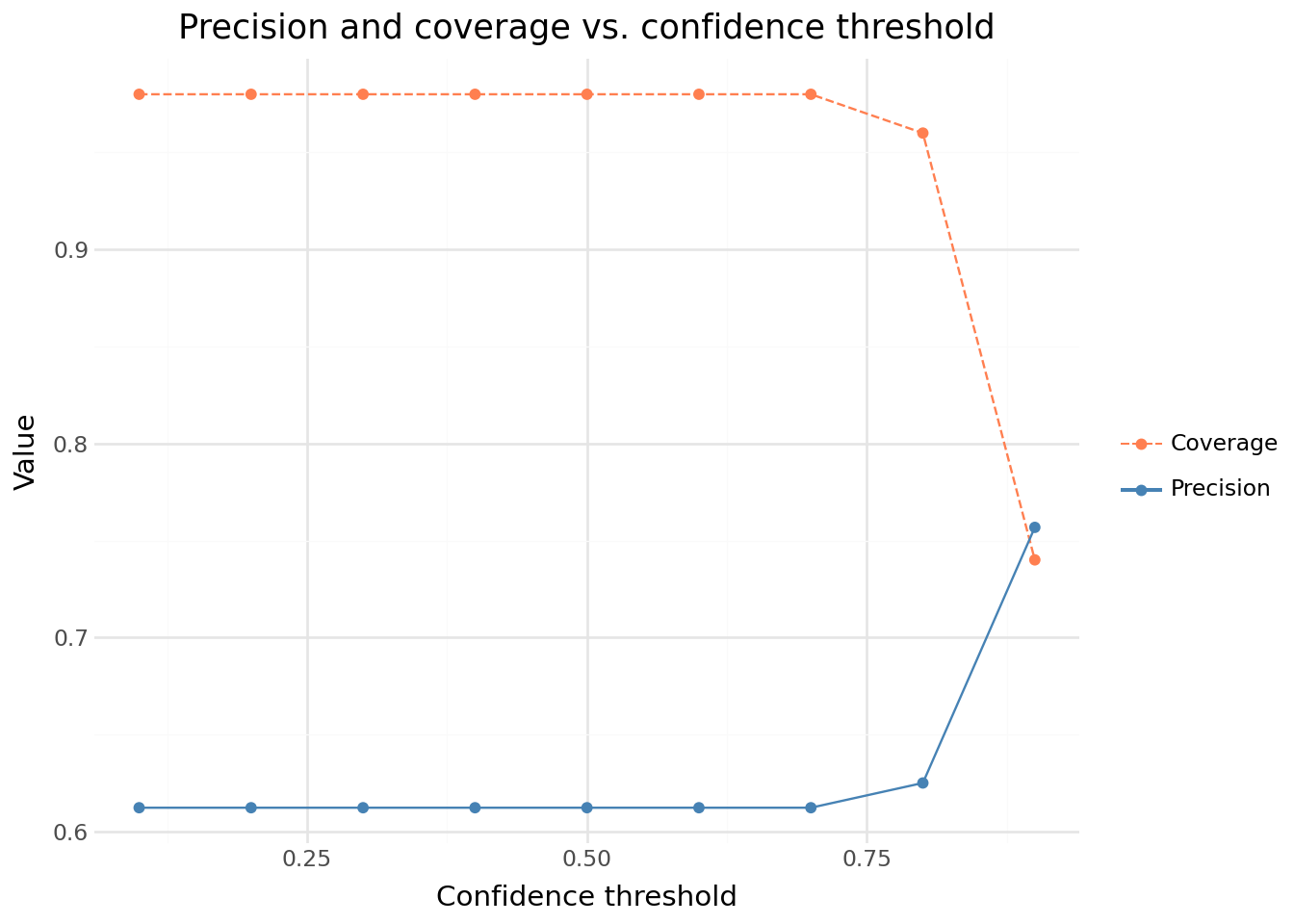
Question 5 — Confidence score analysis
The LLM returns a confidence score with each prediction. In production, this score can serve as a quality signal to filter out unreliable predictions — at the cost of reduced coverage (fewer activities are automatically coded, the rest going to manual review).
Produce two complementary plots to investigate this trade-off:
- A boxplot of the confidence score, split by prediction correctness (correct vs. incorrect). Does the LLM assign higher confidence to predictions that turn out to be correct?
- A precision–coverage curve as a function of the confidence threshold. For each threshold
t ∈ {0.1, 0.2, ..., 0.9}, compute:
- precision: accuracy on the subset of predictions with
confidence ≥ t - coverage: share of the dataset that survives the threshold
- A precision–coverage curve as a function of the confidence threshold. For each threshold
What confidence threshold would you choose if you wanted at least 95% precision? What coverage do you get?
Click to see the answer
from plotnine import (
    ggplot, aes,
    geom_boxplot, geom_line, geom_point,
    scale_color_manual, scale_linetype_manual,
    labs, theme_minimal,
)


# --- Left: confidence distribution by correctness ---
results_plot = results.assign(
    correctness=results["pipeline_correct"].map({False: "Incorrect", True: "Correct"})
)

p1 = (
    ggplot(results_plot, aes(x="correctness", y="confidence"))
    + geom_boxplot()
    + labs(
        title="Confidence distribution by pipeline correctness",
        x="Prediction correct",
        y="Confidence score",
    )
    + theme_minimal()
)

# --- Right: precision and coverage vs confidence threshold ---
thresholds = [i / 10 for i in range(1, 10)]
rows = []
for t in thresholds:
    subset = results[results["confidence"] >= t]
    if len(subset) > 0:
        rows += [
            {"threshold": t, "metric": "Precision", "value": subset["pipeline_correct"].mean()},
            {"threshold": t, "metric": "Coverage",  "value": len(subset) / len(results)},
        ]

df_thresh = pd.DataFrame(rows)

p2 = (
    ggplot(df_thresh, aes(x="threshold", y="value", color="metric", linetype="metric"))
    + geom_line()
    + geom_point()
    + scale_color_manual(values={"Precision": "steelblue", "Coverage": "coral"})
    + scale_linetype_manual(values={"Precision": "solid", "Coverage": "dashed"})
    + labs(
        title="Precision and coverage vs. confidence threshold",
        x="Confidence threshold",
        y="Value",
        color="",
        linetype="",
    )
    + theme_minimal()
)

from IPython.display import display
display(p1)
display(p2)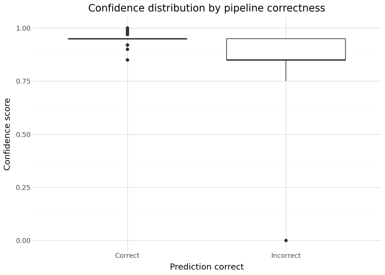
Note
Precision / coverage trade-off: raising the confidence threshold increases precision (the retained predictions are more likely to be correct) but reduces coverage (fewer labels are automatically coded, the rest requiring manual review). Choosing the right threshold depends on the operational constraints of your use case.
TipUsing Polars
You can try avoid using lists and use Polars package instead to do all of the previous steps.
Here is an example for the retrieval step, to search for NACE candidates using Polars’s usefull .unnest() method.
points_df = (
    pl.DataFrame(points.model_dump())
    .unnest()
    .unnest()
    .select(["id", "score", "code", "text"])
)
You can also use Polars in the full pipeline, although it raises some question if you want to put it in production.
def run_rag_pipeline(activity: str) -> dict:
    """
    Run the full RAG pipeline for a single activity label.

    Parameters
    ----------
    activity : str
        Free-text economic activity label to be coded.

    Returns
    -------
    dict with keys:
        - nace_code (str | None) : predicted NACE code
        - codable (bool)        : True if the label could be coded
        - confidence (float)    : confidence score (0–1)
        - retrieved_codes (list): candidates returned by the retriever
    """
    # --- Step 1: Embedding ---
    emb_response = client_llmlab.embeddings.create(model=EMB_MODEL_NAME, input=activity)
    embedding = emb_response.data[0].embedding

    # --- Step 2: Retrieval ---
    points = client_qdrant.query_points(
        collection_name=COLLECTION_NAME,
        query=embedding,
        limit=RETRIEVER_LIMIT,
    )

    points_df = (
        pl.DataFrame(points.model_dump(), schema_overrides={"points": pl.Struct})
        .unnest()
        .unnest()
        .select(["id", "score", "code", "text"])
    )

    # --- Step 3: Prompt construction ---
    user_prompt = USER_PROMPT_TEMPLATE.format(
        activity=activity,
        proposed_nace_descriptions="## " + "\n\n## ".join(points_df["text"]),
        proposed_nace_codes=", ".join(points_df["code"]),
    )

    # --- Step 4: LLM inference ---
    gen_response = client_llmlab.chat.completions.create(
        model=GEN_MODEL_NAME,
        messages=[
            {"role": "system", "content": SYSTEM_PROMPT},
            {"role": "user", "content": user_prompt},
        ],
        temperature=TEMPERATURE,
        response_format={"type": "json_object"},
    )

    result = json.loads(gen_response.choices[0].message.content)
    # Keep retrieved candidates for retriever evaluation
    result["retrieved_codes"] = points_df["code"]

    return result


annotations_df = pl.DataFrame(annotations)

results_df = annotations_df.with_columns(
    pl.col("label")
    .map_elements(
        lambda a: run_rag_pipeline(a),
        return_dtype=pl.Struct(
            {
                "nace_code": pl.Utf8,
                "codable": pl.Boolean,
                "confidence": pl.Float64,
                "retrieved_codes": pl.List(pl.Utf8),
            }
        ),
    )
    .alias("pred")
).unnest()

# Metrics
results_df = (
    results_df.with_columns(
        retriever_hit=pl.col("code").is_in(pl.col("retrieved_codes")),
        pipeline_correct=pl.col("code") == pl.col("nace_code"),
    )
    .with_columns(
        pipeline_correct=pl.col("pipeline_correct").fill_null(
            False  # if no prediction - pipeline is false
        )
    )
    .with_columns(
        llm_correct_given_retriever=pl.when(pl.col("retriever_hit"))
        .then(pl.col("pipeline_correct"))
        .otherwise(None),
    )
)

# Q1
results_df["retriever_hit"].value_counts()
retriever_accuracy = results_df["retriever_hit"].mean()

# Q2
results_df["llm_correct_given_retriever"].value_counts()
results_df.filter(pl.col("retriever_hit"))["llm_correct_given_retriever"].value_counts()
llm_accuracy = results_df.filter(pl.col("retriever_hit"))[
    "llm_correct_given_retriever"
].mean()

# Q3
results_df["pipeline_correct"].value_counts()
pipeline_accuracy = results_df["pipeline_correct"].mean()
pipeline_accuracy
llm_accuracy * retriever_accuracy

# Q4
n_total = len(results_df)

n_retriever_miss = (
    results_df["retriever_hit"]
    .value_counts()
    .filter(~pl.col("retriever_hit"))["count"][0]
)
n_llm_miss = (
    results_df["llm_correct_given_retriever"]
    .value_counts()
    .filter(~pl.col("llm_correct_given_retriever"))["count"][0]
)

n_correct = (
    results_df["pipeline_correct"]
    .value_counts()
    .filter(pl.col("pipeline_correct"))["count"][0]
)
What you learned — and how to go further
Key concepts of the RAG approach
Across the two RAG tutorials you built a complete pipeline from raw text to a coded NACE label:
- Vector database (tutorial 1): NACE definitions were cleaned, embedded with a dense model, and stored in Qdrant as
PointStructobjects with deterministic UUIDs. The choice of embedding model and the richness of the stored text (includes, excludes) directly shape retrieval quality. - Semantic retrieval: at inference time, the activity label is embedded with the same model and the
knearest neighbours are fetched from Qdrant. Retriever@k is the hard ceiling of the pipeline — if the correct code is not retrieved, the LLM cannot recover it. - Structured generation: the retrieved candidates are injected into a prompt and the LLM is asked to pick one, returning a typed
NaceClassificationResultobject viabeta.chat.completions.parse(). Pydantic constraints catch malformed responses at parse time. - Decomposed evaluation: pipeline accuracy factors as Retriever@k × LLM accuracy (conditional). This decomposition pinpoints where errors occur and guides improvements.
- Confidence-based triage: the LLM confidence score enables a precision/coverage trade-off — high-confidence predictions are sent to automatic coding, low-confidence ones to human review.
What to try next
Improve the retriever
- Larger or domain-adapted embedding model: a model fine-tuned on economic activity descriptions would produce better semantic clusters than a general-purpose one.
- Hybrid search: combine dense (embedding) and sparse (BM25 keyword) search. Qdrant supports this natively. Useful when the activity label contains exact NACE terminology.
- Increase k and rerank: retrieve more candidates (e.g.
k=10) and add a lightweight cross-encoder reranker to re-score them before passing the top-5 to the LLM. Rerankers are better at fine-grained relevance but too slow to run over the full collection.
Improve the generator
- Few-shot examples in the prompt: add 2–3 labelled examples (activity → code) to the user prompt. This helps the LLM calibrate on the expected granularity of the nomenclature.
- Chain-of-thought: ask the LLM to reason step-by-step before outputting the JSON. Adds latency but can improve accuracy on ambiguous labels.
- More capable model: swap
GEN_MODEL_NAMEfor a larger or instruction-tuned model — generation errors are usually the cheaper component to improve.
Better evaluation
- Hierarchical accuracy: count a prediction as partially correct if it matches the true code at the section or division level (e.g.
47matches47.11). This is more informative than strict exact-match for a 4-level hierarchy. - Larger evaluation set:
SAMPLE_SIZE = 100gives noisy estimates. Run on the full dataset or use bootstrap confidence intervals. - Error analysis by sector: accuracy may vary widely across NACE sections. Identifying weak sectors guides targeted improvements.
Production considerations
- Caching embeddings: if the same activity labels recur (e.g. standard job titles), cache their embeddings to avoid redundant API calls.
- Async batching: parallelise the embedding + generation calls with
asyncioto reduce wall-clock time on large batches. - Human-in-the-loop: route low-confidence predictions (
confidence < t) to a review queue rather than discarding them — combine automatic coding with human validation to maximise both precision and coverage.