Data acquisition

Where this chapter fits

Training a segmentation model needs a dataset of (image, label) pairs — satellite tiles on one side, land-cover maps on the other. This chapter builds that dataset. By the end, you’ll know how to pull a Sentinel-2 tile for any European city, fetch its matching CLC + label (Corinne Land Cover), and confirm the two are perfectly aligned pixel-for-pixel.

flowchart LR
    C1["Chapter 1Build the(image, label) dataset"]:::current
    C2["Chapter 2 (optional)Train a model on the dataset"]
    C3["Chapter 3Use a trained modelto predict new masks"]
    C4["Chapter 4Compute regionalland-cover statistics"]
    C1 --> C2 --> C3 --> C4
    classDef current fill:#fde68a,stroke:#b45309,stroke-width:2px;

You don’t need any machine learning knowledge to complete this chapter — it’s all about reading satellite rasters, handling geographic coordinates, and pairing images with their labels.

What you will learn in this chapter

Manipulating satellite imagery — load multispectral Sentinel-2 rasters with rasterio, display RGB and false-colour composites, compute vegetation indices (NDVI)
Working with geographic data — use coordinate reference systems (CRS), build geometries with shapely, perform spatial joins and interactive mapping with GeoPandas and Folium
Building a training dataset — pair Sentinel-2 images with CLC+ Backbone land-cover labels to create the input/target pairs needed to train a segmentation model
(Optional) Acquiring new data from APIs — query the Copernicus Data Space Ecosystem via Sentinel Hub and OData APIs

1 Sentinel-2 — Understanding and Visualizing Satellite Imagery

This section introduces Sentinel-2 satellite imagery and teaches you how to load, explore, and display multispectral raster data in Python. We start with a single local file — no cloud storage or URL patterns yet — so you can focus entirely on understanding how satellite images work.

1.1 What is Sentinel-2?

Sentinel-2 is an Earth observation mission from the European Space Agency (ESA), part of the Copernicus programme. It consists of two twin satellites — Sentinel-2A and Sentinel-2B — placed in the same sun-synchronous orbit but phased 180 degrees apart, giving a 5-day revisit time at the equator.

Key characteristics:

13 spectral bands spanning visible, near-infrared (NIR) and short-wave infrared (SWIR)
Spatial resolution of 10 m, 20 m or 60 m depending on the band
290 km swath width
Free and open data policy

These properties make Sentinel-2 a reference dataset for land-cover mapping, agricultural monitoring, forestry, urban change detection and many other applications.

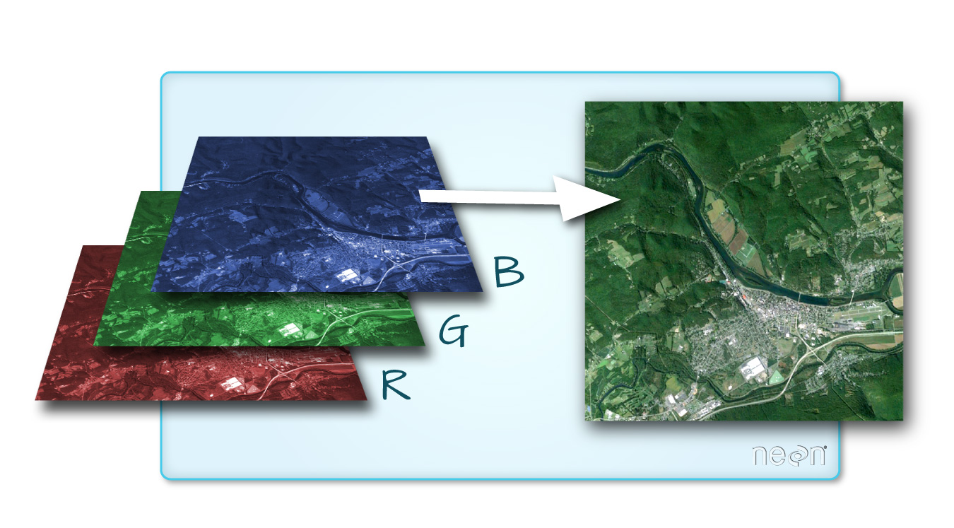
Why multiple bands matter. A regular camera captures three channels (Red, Green, Blue). Sentinel-2 captures 13 channels at different wavelengths — from visible light to short-wave infrared. Each band reveals different properties of the surface: vegetation health, water content, bare soil, etc. By combining bands in different ways, we can extract information that is invisible to the naked eye.

The Twin-Satellite Sentinel-2 Orbital Configuration (Credits: Astrium GmbH)

Tip

Learn more: Sentinel-2 Mission information (see in particular the Sentinel-2 Spectral Response Functions (S2-SRF) document for the spectral bands) · Sentinel Hub custom scripts gallery

1.1.1 Spectral bands

A spectral band is a narrow window of wavelengths that the sensor records separately. Sentinel-2’s MultiSpectral Instrument (MSI) captures 13 bands spanning visible, near-infrared (NIR) and short-wave infrared (SWIR) light — from 443 nm to 2190 nm. Each band is tuned to a specific physical property of the surface or atmosphere, and the table below groups them by native spatial resolution, which reflects a hardware trade-off made by ESA:

10 m — the “core” mapping bands. B2 (blue), B3 (green), B4 (red) and B8 (NIR). These are the bands you’ll use most often to look at the landscape: true-colour RGB composites, NDVI, and any high-detail analysis of vegetation, water or built-up areas.
20 m — vegetation structure and moisture. The three red-edge bands (B5, B6, B7) trace the steep transition between red and NIR that is characteristic of healthy chlorophyll. B8A is a narrower NIR window, and B11/B12 (SWIR) are sensitive to water content in leaves and soil, as well as snow/cloud discrimination.
60 m — atmospheric correction. B1 (coastal aerosol), B9 (water vapour) and B10 (cirrus). These bands exist primarily to clean up the other bands, not to describe the ground, so a coarser pixel is sufficient.

Note

L1C vs L2A — two processing levels. Copernicus distributes Sentinel-2 data at two processing levels. Level-1C contains top-of-atmosphere reflectance for all 13 bands. Level-2A applies atmospheric correction and delivers surface reflectance, which is what we want for land-cover mapping. L2A drops B10 (the cirrus band — only useful for cloud detection, not for the surface) and delivers 12 spectral bands. The training dataset in this tutorial is built from L2A products: the pre-processed GeoTIFFs stack these 12 spectral bands and append two derived vegetation/water indices, NDVI and NDWI, for a total of 14 channels.

A GeoTIFF is a standard TIFF image file with extra embedded metadata describing where the image sits on Earth — coordinate reference system (CRS), pixel size, and an affine transform that maps each (row, column) to a geographic (x, y) coordinate. In other words: a regular image plus the spatial information needed to overlay it correctly on a map. The format also supports multiple bands in a single file, which is why we can pack the 14 channels into one .tif

NDVI (Normalised Difference Vegetation Index) and NDWI (Normalised Difference Water Index) are computed once at preprocessing time so the model can use them as input features without having to re-derive them from the spectral bands at every batch.

src/download_region.py follows the same convention and produces 14-channel float64 GeoTIFFs identical in layout to those on projet-funathon.

Band	Central wavelength (nm)	Resolution (m)	Description	Use / Application
B1	443	60	Coastal aerosol	Detects aerosols and haze; used for atmospheric correction over coastal waters.
B2	490	10	Blue	Visible blue channel; useful for bathymetry and distinguishing soil from vegetation.
B3	560	10	Green	Peak vegetation reflectance; also used for water body delineation.
B4	665	10	Red	Chlorophyll absorption; key band for computing NDVI and monitoring vegetation health.
B5	705	20	Vegetation red edge	Sensitive transition zone between red and NIR; indicates chlorophyll content and vegetation stress.
B6	740	20	Vegetation red edge	Refines canopy chlorophyll estimation and leaf area index mapping.
B7	783	20	Vegetation red edge	Captures the full red-edge slope for detailed vegetation structure analysis.
B8	842	10	NIR	Strongly reflected by healthy vegetation; the primary NIR band used in NDVI.
B8A	865	20	Narrow NIR	Narrower NIR window for more precise vegetation and land-surface reflectance studies.
B9	945	60	Water vapour	Measures atmospheric water vapour column; used for atmospheric correction.
B10	1375	60	SWIR – Cirrus	Detects thin cirrus clouds; used for cloud masking before analysis.
B11	1610	20	SWIR	Sensitive to vegetation water content and soil moisture; discriminates snow from clouds.
B12	2190	20	SWIR	Detects dry/senescent vegetation, differentiates geological materials, and maps burn severity.

1.2 What is rasterio?

rasterio is a Python library built on top of GDAL for reading and writing geospatial raster data (GeoTIFF, etc.). It is the standard tool for working with satellite imagery in Python.

Note

Think of a raster as a spreadsheet with coordinates. A regular spreadsheet has rows and columns filled with numbers. A raster is the same idea, except each cell is a pixel located at a specific place on Earth, and you can stack multiple layers (bands) on top of each other — one layer per spectral band.

Single-band vs. multi-band raster. *Source: Earth Lab — Earth Data Science (CC BY-SA 4.0) / NEON.*

Key concepts:

Raster = a grid of pixels organised into bands (layers). Each band represents one channel of data (e.g. a spectral band from a satellite sensor).
rasterio.open(path) returns a DatasetReader — works with local files and HTTPS URLs alike.
src.read(bands) returns a NumPy array with shape (bands, H, W) — this is the CHW (Channel, Height, Width) convention, used by rasterio, PyTorch, and most deep learning frameworks. For display with matplotlib (or PIL), you need to transpose to (H, W, C) — the HWC (Height, Width, Channel) convention — using np.transpose(array, (1, 2, 0)). Expect to move between the two conventions constantly: CHW when feeding arrays to a model, HWC when plotting them.
src.crs — the coordinate reference system attached to the raster.
src.bounds — the geographic extent as (left, bottom, right, top).
src.profile / src.meta — full metadata dictionary (driver, dtype, nodata value, affine transform, etc.).

Why band indexing matters: Sentinel-2 has 13 spectral bands, reading specific band combinations reveals different features:

src.read([4, 3, 2]) → true-colour RGB (Red, Green, Blue)
src.read([8, 4, 3]) → false-colour composite (NIR, Red, Green) — vegetation appears bright red
src.read([8, 4]) → bands needed for NDVI (Normalised Difference Vegetation Index)

You will practise these combinations in the exercises below.

Warning

Watch out: rasterio band index ≠ Sentinel-2 band number. In the pre-processed GeoTIFFs the channel layout is:

Rasterio index	1	2	3	4	5	6	7	8	9	10	11	12	13	14
Content	B1	B2	B3	B4	B5	B6	B7	B8	B8A	B9	B11	B12	NDVI	NDWI

Two things to remember:

B8A sits at index 9, before B9. So src.read(9) returns narrow NIR (B8A), not B9. It is only a coincidence that src.read(2) through src.read(8) line up with B2–B8.
There is no B10 in the file. L2A processing removes it (cirrus band, no surface information), so index 11 jumps straight to B11. Indices 13 and 14 are NDVI and NDWI, computed once during preprocessing.

Check this table before adapting code for SWIR (B11, B12) or the derived indices to avoid off-by-one bugs.

Tip

Learn more: rasterio documentation

1.3 Loading a Sentinel-2 tile

For this tutorial, we work with pre-processed Sentinel-2 patches that are publicly available on sspcloud object storage. To keep things simple at this stage, we download a single sample tile of a completely random location and work with it directly.

import os
import urllib.request
import rasterio
import numpy as np

tile_url = (
    "https://minio.lab.sspcloud.fr/projet-funathon/2026/"
    "project3/data/images/LU000/"
    "2024/4042000_2951690_0_637.tif"
)

with rasterio.open(tile_url) as src:
    tile_crs = src.crs
    tile_bounds = src.bounds
    tile_count = src.count
    tile_height = src.height
    tile_width = src.width
    # Read RGB bands: B4 (Red), B3 (Green), B2 (Blue)
    rgb_data = src.read([4, 3, 2])

print(f"CRS:    {tile_crs}")
print(f"Bounds: {tile_bounds}")
print(f"Shape:  {tile_count} bands x {tile_height} x {tile_width} px")

CRS:    EPSG:3035
Bounds: BoundingBox(left=4042000.0, bottom=2951690.0, right=4044500.0, top=2954190.0)
Shape:  14 bands x 250 x 250 px

Note

The pre-processed GeoTIFF files used here contain 14 channels: the 12 L2A spectral bands (B01–B12 with B10 dropped, plus B8A) in bands 1–12, then NDVI as band 13 and NDWI as band 14. NDVI and NDWI are derived vegetation/water indices — they’re not spectral bands but cheap, useful features the model receives directly.

Now let’s display the tile as an RGB composite (true-colour: Red, Green, Blue).

A quick word on display normalization. Raw Sentinel-2 L2A surface reflectance is stored as 16-bit integers on a 0–10 000 scale. matplotlib expects RGB values in [0, 1], so passing the raw array directly produces an almost-black image. We fix this with a standard percent-clip contrast stretch: divide every pixel by the 98th percentile of the image (so ~98 % of pixels fall into [0, 1]) and then clamp the top 2 % to 1. This is the same idea as the “percent clip” stretch in QGIS or ArcGIS — it’s robust to the handful of extremely bright outliers (clouds, specular reflections, sensor artefacts) that would otherwise compress the rest of the image into a dark band.

#

import matplotlib.pyplot as plt

# Transpose to (H, W, 3) and normalize for display
rgb = np.transpose(rgb_data, (1, 2, 0)).astype(np.float32)
p98 = np.percentile(rgb, 98)
rgb = np.clip(rgb / p98, 0, 1)

fig, ax = plt.subplots(figsize=(5, 5))
ax.imshow(rgb)
ax.set_title("Sentinel-2 RGB composite (B4, B3, B2) — LU000")
ax.axis("off")
plt.tight_layout()
plt.show()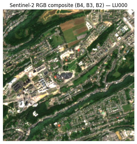

Line-by-line breakdown (and what happens without normalization)

np.transpose(rgb_data, (1, 2, 0)) — rearranges from rasterio’s (bands, height, width) to matplotlib’s expected (height, width, bands).
np.percentile(rgb, 98) — the 98th percentile of all pixel values, used instead of the true maximum so that a few bright outliers don’t dominate the scale.
np.clip(rgb / p98, 0, 1) — rescales so ~98 % of pixels fall into [0, 1] and clamps the top 2 % to white.

Without those three lines, the raw 16-bit data displays like this:

import matplotlib.pyplot as plt

# Transpose to (H, W, 3) and normalize for display
rgb = np.transpose(rgb_data, (1, 2, 0)).astype(np.float32)

fig, ax = plt.subplots(figsize=(5, 5))
ax.imshow(rgb)
ax.set_title("Sentinel-2 RGB composite (B4, B3, B2) — LU000 (no normalization)")
ax.axis("off")
plt.tight_layout()
plt.show()

Exercise 1 — Read a Sentinel-2 tile and display it

Goal: Open the remote sample Sentinel-2 patch, extract the RGB bands, normalize the image, and display it.

Steps:

Open the tile with rasterio.open(tile_url) and read bands 4, 3, 2 (Red, Green, Blue)
Store the CRS and bounds from the rasterio source
Transpose the array to (H, W, 3) and normalize for display (divide by the 98th percentile, clip to [0, 1])
Display the RGB composite with matplotlib

Hint — Exercise 1

Inside the with rasterio.open(tile_url) as src: block, use src.read([4, 3, 2]) to get a (3, H, W) array.
src.crs and src.bounds give you the CRS and bounding box.
Transpose with np.transpose(rgb_data, (1, 2, 0)), cast to float32, then normalize: divide by np.percentile(rgb, 98) and clip to [0, 1] with np.clip.

Code template:

import rasterio
import numpy as np
import matplotlib.pyplot as plt

tile_url = (
    "https://minio.lab.sspcloud.fr/projet-funathon/2026/"
    "project3/data/images/LU000/"
    "2024/4042000_2951690_0_637.tif"
)

# Step 1: Open the tile and read RGB bands (4, 3, 2)
with rasterio.open(tile_url) as src:
    rgb_data = ___  # TODO: read bands 4, 3, 2
    tile_crs = ___  # TODO
    tile_bounds = ___  # TODO

# Step 2: Transpose to (H, W, 3) and normalize
rgb = ___  # TODO: np.transpose, then normalize with 98th percentile and clip

# Step 3: Display
fig, ax = plt.subplots(figsize=(5, 5))
___  # TODO: ax.imshow(...)
ax.set_title("Sentinel-2 RGB composite")
ax.axis("off")
plt.tight_layout()
plt.show()

Solution — Exercise 1

import rasterio
import numpy as np
import matplotlib.pyplot as plt

tile_url = (
    "https://minio.lab.sspcloud.fr/projet-funathon/2026/"
    "project3/data/images/LU000/"
    "2024/4042000_2951690_0_637.tif"
)

with rasterio.open(tile_url) as src:
    rgb_data = src.read([4, 3, 2])
    tile_crs = src.crs
    tile_bounds = src.bounds

rgb = np.transpose(rgb_data, (1, 2, 0)).astype(np.float32)
p98 = np.percentile(rgb, 98)
rgb = np.clip(rgb / p98, 0, 1)

fig, ax = plt.subplots(figsize=(5, 5))
ax.imshow(rgb)
ax.set_title("Sentinel-2 RGB composite")
ax.axis("off")
plt.tight_layout()
plt.show()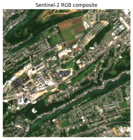

1.4 What are band composites?

A band composite is an image formed by mapping three spectral bands to the Red, Green, and Blue channels of a display. By choosing different bands, you highlight different surface properties:

True-colour (B4, B3, B2) — what the human eye would see. Useful for general orientation.
False-colour (B8, B4, B3) — near-infrared mapped to red. Healthy vegetation appears bright red because it strongly reflects NIR light. Useful for spotting vegetation stress, urban areas, and water bodies.
NDVI (Normalised Difference Vegetation Index) — not a composite, but a single-band index computed from NIR and Red: $\text{NDVI} = \frac{B8 - B4}{B8 + B4}$. Values near +1 indicate dense vegetation; near 0 indicate bare soil; negative values indicate water.

Tip

Learn more: Wikipedia — NDVI · Sentinel Hub custom scripts gallery

Exercise 2 — Explore raster metadata and create a false-colour composite

Goal: Inspect the raster metadata of a Sentinel-2 tile using src.profile, then create a false-colour composite using bands 8 (NIR), 4 (Red), 3 (Green).

Steps:

Open the tile with rasterio.open(tile_url) and print src.profile
Read bands [8, 4, 3] (NIR, Red, Green)
Normalize the false-colour image (same method as Exercise 1: 98th percentile + clip)
Display the true-colour RGB (from Exercise 1) and false-colour composite side by side

Hint — Exercise 2

src.profile is a dictionary — just print(src.profile) to see driver, dtype, crs, transform, etc.
src.read([8, 4, 3]) reads NIR, Red, Green in that order → shape (3, H, W).
Normalize exactly as in Exercise 1: transpose to (H, W, 3), divide by np.percentile(fc, 98), clip to [0, 1].

Code template:

import rasterio
import numpy as np
import matplotlib.pyplot as plt

tile_url = (
    "https://minio.lab.sspcloud.fr/projet-funathon/2026/"
    "project3/data/images/LU000/"
    "2024/4042000_2951690_0_637.tif"
)

# Step 2a: Open the tile and print the raster profile
with rasterio.open(tile_url) as src:
    print(___) # TODO: print src.profile

    # Step 2b: Read false-colour bands (NIR=8, Red=4, Green=3)
    fc_data = ___  # TODO: src.read([8, 4, 3])

# Step 2c: Normalize for display
fc = np.transpose(fc_data, (1, 2, 0)).astype(np.float32)
p98 = ___  # TODO: np.percentile(fc, 98)
fc = ___   # TODO: np.clip(fc / p98, 0, 1)

# Step 2d: Display side by side with the true-colour RGB
fig, axes = plt.subplots(1, 2, figsize=(10, 5))
axes[0].imshow(rgb)
axes[0].set_title("True colour (B4, B3, B2)")
axes[0].axis("off")
___  # TODO: axes[1].imshow(fc)
axes[1].set_title("False colour (B8, B4, B3)")
axes[1].axis("off")
plt.tight_layout()
plt.show()

Solution — Exercise 2

import rasterio
import numpy as np
import matplotlib.pyplot as plt

tile_url = (
    "https://minio.lab.sspcloud.fr/projet-funathon/2026/"
    "project3/data/images/LU000/"
    "2024/4042000_2951690_0_637.tif"
)

with rasterio.open(tile_url) as src:
    print(src.profile)
    fc_data = src.read([8, 4, 3])

fc = np.transpose(fc_data, (1, 2, 0)).astype(np.float32)
p98 = np.percentile(fc, 98)
fc = np.clip(fc / p98, 0, 1)

fig, axes = plt.subplots(1, 2, figsize=(10, 5))
axes[0].imshow(rgb)
axes[0].set_title("True colour (B4, B3, B2)")
axes[0].axis("off")
axes[1].imshow(fc)
axes[1].set_title("False colour (B8, B4, B3)")
axes[1].axis("off")
plt.tight_layout()
plt.show()

{'driver': 'GTiff', 'dtype': 'float64', 'nodata': None, 'width': 250, 'height': 250, 'count': 14, 'crs': CRS.from_wkt('PROJCS["ETRS89-extended / LAEA Europe",GEOGCS["ETRS89",DATUM["European_Terrestrial_Reference_System_1989",SPHEROID["GRS 1980",6378137,298.257222101,AUTHORITY["EPSG","7019"]],AUTHORITY["EPSG","6258"]],PRIMEM["Greenwich",0,AUTHORITY["EPSG","8901"]],UNIT["degree",0.0174532925199433,AUTHORITY["EPSG","9122"]],AUTHORITY["EPSG","4258"]],PROJECTION["Lambert_Azimuthal_Equal_Area"],PARAMETER["latitude_of_center",52],PARAMETER["longitude_of_center",10],PARAMETER["false_easting",4321000],PARAMETER["false_northing",3210000],UNIT["metre",1,AUTHORITY["EPSG","9001"]],AXIS["Northing",NORTH],AXIS["Easting",EAST],AUTHORITY["EPSG","3035"]]'), 'transform': Affine(10.0, 0.0, 4042000.0,
       0.0, -10.0, 2954190.0), 'blockxsize': 250, 'blockysize': 1, 'tiled': False, 'interleave': 'pixel'}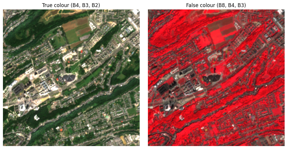

Exercise 3 — Compute and display NDVI

Goal: Compute the Normalised Difference Vegetation Index (NDVI) from a Sentinel-2 tile and display it as a colour-coded map.

NDVI is defined as:

\[ \text{NDVI} = \frac{\text{NIR} - \text{Red}}{\text{NIR} + \text{Red}} \]

NDVI values range from −1 to +1:

Near +1 → dense, healthy vegetation
Near 0 → bare soil, urban areas
Negative → water bodies

Steps:

Read bands 8 (NIR) and 4 (Red) as float32
Compute NDVI pixel-wise, handling division by zero
Display with imshow(cmap="RdYlGn", vmin=-1, vmax=1) and a colorbar

Hint — Exercise 3

src.read(8) reads a single band → shape (H, W). Cast to float32 for division.
Use np.where(nir + red == 0, 0, (nir - red) / (nir + red)) to avoid division by zero.
cmap="RdYlGn" gives a red-yellow-green colour scale: red for low NDVI, green for high.
fig.colorbar(im, ax=ax, shrink=0.8, label="NDVI") adds a colour legend.

Code template:

import rasterio
import numpy as np
import matplotlib.pyplot as plt

tile_url = (
    "https://minio.lab.sspcloud.fr/projet-funathon/2026/"
    "project3/data/images/LU000/"
    "2024/4042000_2951690_0_637.tif"
)

# Step 3a: Read NIR (band 8) and Red (band 4) as float32
with rasterio.open(tile_url) as src:
    nir = ___  # TODO: src.read(8).astype(np.float32)
    red = ___  # TODO: src.read(4).astype(np.float32)

# Step 3b: Compute NDVI (handle division by zero)
ndvi = ___  # TODO: np.where(nir + red == 0, 0, (nir - red) / (nir + red))

# Step 3c: Display
fig, ax = plt.subplots(figsize=(6, 5))
im = ___  # TODO: ax.imshow(ndvi, cmap="RdYlGn", vmin=-1, vmax=1)
ax.set_title("NDVI — LU000 (2024)")
ax.axis("off")
___  # TODO: fig.colorbar(im, ax=ax, shrink=0.8, label="NDVI")
plt.tight_layout()
plt.show()

Solution — Exercise 3

import rasterio
import numpy as np
import matplotlib.pyplot as plt

tile_url = (
    "https://minio.lab.sspcloud.fr/projet-funathon/2026/"
    "project3/data/images/LU000/"
    "2024/4042000_2951690_0_637.tif"
)

with rasterio.open(tile_url) as src:
    # Healthy vegetation strongly reflects near-infrared (B8) and absorbs red (B4),
    # so the ratio (NIR − Red) / (NIR + Red) gives a clean vegetation signal.
    nir = src.read(8).astype(np.float32)
    red = src.read(4).astype(np.float32)

# np.where guards against pixels where NIR + Red is exactly 0 (water bodies,
# nodata, deep shadow): the ratio would otherwise produce NaN and contaminate the
# colormap. Substituting 0 keeps those pixels neutral on the red-yellow-green scale.
ndvi = np.where(nir + red == 0, 0, (nir - red) / (nir + red))

fig, ax = plt.subplots(figsize=(6, 5))
# vmin=-1, vmax=1 anchors the colormap to NDVI's full theoretical range, so the
# same colour means the same vegetation cover across tiles.
im = ax.imshow(ndvi, cmap="RdYlGn", vmin=-1, vmax=1)
ax.set_title("NDVI — LU000 (2024)")
ax.axis("off")
fig.colorbar(im, ax=ax, shrink=0.8, label="NDVI")
plt.tight_layout()
plt.show()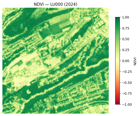

2 NUTS Regions and Finding Satellite Tiles

Now that you know how to read and display a single satellite image, the next question is: how do you find the right image for a given location? The pre-processed tiles in this project are organized by NUTS region. This section explains what NUTS regions are, how tile URLs are structured, and how to go from a city name to the correct tile.

2.1 What are NUTS regions?

NUTS (Nomenclature of Territorial Units for Statistics) is a hierarchical classification of administrative regions used by Eurostat for statistical purposes across Europe. The hierarchy has four levels:

Level	Granularity	Example (France / Paris)	Example name
NUTS 0	Country	`FR`	France
NUTS 1	Major region	`FR1`	Île-de-France
NUTS 2	Region	`FR10`	Île-de-France
NUTS 3	Province / department	`FR101`	Paris

In this project, data is organized at the NUTS 3 level — each satellite tile belongs to a specific NUTS3 region. The NUTS3 code appears in the file path and URL.

NUTS boundaries are published as open data by GISCO (Eurostat’s geographic information system) in GeoJSON and other formats.

Tip

Learn more: Eurostat NUTS overview · GISCO distribution API

2.2 How data is organized on S3

Pre-processed Sentinel-2 patches are publicly available on the SSP Cloud object storage. You can access them over HTTPS (no authentication required) or via S3 (with credentials).

The HTTPS URL follows this pattern:

https://minio.lab.sspcloud.fr/projet-funathon/2026/project3/data/images/{NUTS}/{year}/{patch_id}.tif

The equivalent S3 path is:

s3://projet-funathon/2026/project3/data/images/{NUTS}/{year}/{patch_id}.tif

Each pre-processed patch is a GeoTIFF covering a 250 x 250 pixel area (2 500 m at 10 m resolution). That size is a practical compromise: large enough to give the segmentation model meaningful spatial context (parcel boundaries, roads, forest edges, river meanders), small enough to fit many patches per GPU batch during training, and small enough that a whole NUTS3 region can be tiled into a few hundred patches rather than a few million. The URL path encodes the key metadata:

...images/{NUTS}/{year}/{xmin}_{ymin}_{idx}_{id}.tif

Field	Example value	Meaning
NUTS	`LU000`	NUTS-3 region (Luxembourg)
year	`2024`	Acquisition year
xmin, ymin	`4042000`,`2951690`	Lower-left corner in EPSG:3035 (metres)

Each {NUTS}/{year}/ directory also contains a filename2bbox.parquet index file that maps every tile filename to its bounding box:

.../images/{NUTS}/{year}/filename2bbox.parquet

This file has two columns: filename (the .tif name) and bbox (a list of four floats [xmin, ymin, xmax, ymax] in EPSG:3035). It lets you find which tile covers a specific location without listing the full directory.

HTTPS vs S3 access

The HTTPS URLs work from anywhere without credentials — great for reading individual tiles with rasterio. The S3 paths require SSP Cloud credentials (AWS_S3_ENDPOINT, AWS_ACCESS_KEY_ID, AWS_SECRET_ACCESS_KEY) but support directory listing and bulk operations via s3fs.

Important

Available regions. Not all NUTS3 regions have pre-processed tiles. The following 27 regions are covered:

NUTS3 Code	Country	Years available
AT332	Austria	2018, 2021, 2024
BE100	Belgium	2018, 2021, 2024
BE251	Belgium	2018, 2021, 2024
BG322	Bulgaria	2018, 2021, 2024
CY000	Cyprus	2021, 2024
CZ072	Czechia	2021, 2024
DEA54	Germany	2018, 2021, 2024
DK041	Denmark	2018, 2024
EE00A	Estonia	2018, 2021, 2024
EL521	Greece	2018, 2021, 2024
ES612	Spain	2018, 2021, 2024
FI1C1	Finland	2018, 2021, 2024
FRJ27	France	2018, 2021, 2024
FRK26	France	2018, 2021, 2024
HR050	Croatia	2018, 2021, 2024
IE061	Ireland	2018, 2021
ITI32	Italy	2018, 2021, 2024
LT028	Lithuania	2018, 2021, 2024
LU000	Luxembourg	2018, 2021, 2024
LV008	Latvia	2018, 2021, 2024
MT001	Malta	2018, 2021, 2024
NL33C	Netherlands	2018, 2021, 2024
PL414	Poland	2018, 2021, 2024
PT16I	Portugal	2018, 2021, 2024
RO123	Romania	2018, 2021, 2024
SE311	Sweden	2018, 2021, 2024
SI035	Slovenia	2018, 2021, 2024
SK022	Slovakia	2018, 2021, 2024
UKJ22	United Kingdom	2018, 2021, 2024
UKRAINE	Ukraine	2018, 2021, 2024

Note

Scale of the dataset and class imbalance. Across the 27 pre-processed NUTS3 regions and the available years (2021 and 2024), the dataset contains roughly 15 000–20 000 (image, label) patches — a comfortable size for training a segmentation model on a single GPU. Because these regions are built around European capital cities, the 10 CLC+ classes are not evenly represented: sealed surfaces, permanent herbaceous and periodically herbaceous dominate, while lichens and mosses or broadleaved evergreen trees are rare or completely absent in most tiles. This class imbalance is a first-order concern when training a segmentation model — naive training will optimise for the common classes and ignore the rare ones.

2.3 Finding a NUTS3 region from a city name

Given a city name, you can geocode it (convert the name to geographic coordinates) and then use a spatial join to find which NUTS3 region it belongs to. The Nominatim API (based on OpenStreetMap data) provides free geocoding.

Here is the complete workflow:

flowchart LR
    A["City name"] --> B["Nominatim API<br>→ (lon, lat) WGS84"]
    B --> C["Reproject<br>EPSG:3035"]
    C --> D["Spatial join<br>with NUTS3"]
    D --> E["NUTS code"]
    E --> F["<pre>filename2bbox.parquet</pre>"]
    F --> G["Tile URL"]

Figure 1: From a city name to a satellite tile URL.

Here is a complete example for the Eurostat headquarters in Luxembourg:

import requests
import geopandas as gpd
from shapely.geometry import Point

# Step 1: Geocode the city name
response = requests.get(
    "https://nominatim.openstreetmap.org/search",
    params={"q": "5, rue Alphonse Weicker  Luxembourg", "format": "json", "limit": 1},
    headers={"User-Agent": "funathon-project3"},
)
result = response.json()[0]
lon, lat = float(result["lon"]), float(result["lat"])
print(f"Eurostat coordinates: lon={lon}, lat={lat}")

# Step 2: Create a GeoDataFrame with the point in WGS84, then reproject
city_point = gpd.GeoDataFrame(
    {"city": ["Luxembourg"]}, geometry=[Point(lon, lat)], crs="EPSG:4326"
)
city_point = city_point.to_crs("EPSG:3035")

# Step 3: Load NUTS3 boundaries and spatial join
nuts_url = (
    "https://gisco-services.ec.europa.eu/distribution/v2/"
    "nuts/geojson/NUTS_RG_01M_2021_3035_LEVL_3.geojson"
)
nuts = gpd.read_file(nuts_url)
city_nuts = gpd.sjoin(city_point, nuts, predicate="within")
nuts_code = city_nuts.iloc[0]["NUTS_ID"]
print(f"NUTS3 region: {nuts_code}")  # → LU000

Eurostat coordinates: lon=6.1695145, lat=49.6335945
NUTS3 region: LU000

Warning

Stay within the supported regions. The code above will compute a NUTS3 code for any city worldwide, but the rest of this notebook — and all the exercises that follow — only have pre-processed tiles for the regions listed in the Available regions table above (e.g. LU000, BE100, FRJ27, …). If your city falls outside those regions, the S3 URL built in the next step will point at an empty prefix and every downstream exercise will fail to load any data. Pick a city inside one of the supported NUTS3 regions before continuing.

Once you have the NUTS3 code, you can build the S3 base URL for tiles in that region:

#| eval: false

base_url = f"s3://projet-funathon/2026/project3/data/images/{nuts_code}"
print(base_url)

Tip

Learn more: Nominatim API docs

Exercise 4 — Geocode a city and build a tile URL

Goal: Pick a city of your choice, find its NUTS3 region via geocoding + spatial join, and build the S3 URL prefix for that region’s tiles.

Steps:

Geocode your chosen city using the Nominatim API
Create a Point(lon, lat) geometry and wrap it in a GeoDataFrame (CRS: EPSG:4326)
Reproject to EPSG:3035 and spatial-join with the NUTS3 boundaries
Check if the resulting NUTS3 code is in the list of available regions
Build the S3 base URL: s3://projet-funathon/2026/project3/data/images/{nuts_code}

Hint — Exercise 4

Nominatim params: {"q": "City, Country", "format": "json", "limit": 1}. Always include a User-Agent header.
Coordinates: Point(lon, lat) — longitude first, latitude second.
Initial CRS is "EPSG:4326" (WGS84), reproject to "EPSG:3035" to match the NUTS3 boundaries.
Use predicate="within" for the spatial join (point inside polygon).
The NUTS3 code column is "NUTS_ID".

Code template:

import requests
import geopandas as gpd
from shapely.geometry import Point

# Step 1: Geocode
response = requests.get(
    "https://nominatim.openstreetmap.org/search",
    params={"q": ___, "format": "json", "limit": 1},  # TODO: city name
    headers={"User-Agent": "funathon-project3"},
)
result = response.json()[0]
lon, lat = ___, ___  # TODO: extract coordinates

# Step 2: Create GeoDataFrame and reproject
city_point = gpd.GeoDataFrame(
    {"city": [___]},
    geometry=[Point(___, ___)],
    crs=___,  # TODO
)
city_point = city_point.to_crs(___)  # TODO: target CRS

# Step 3: Load NUTS3 boundaries and spatial join
nuts_url = (
    "https://gisco-services.ec.europa.eu/distribution/v2/"
    "nuts/geojson/NUTS_RG_01M_2021_3035_LEVL_3.geojson"
)
nuts = gpd.read_file(nuts_url)
city_nuts = gpd.sjoin(___, ___, predicate=___)  # TODO
nuts_code = city_nuts.iloc[0][___]  # TODO: column name

# Step 4: Check availability
available = [
    "AT332",
    "BE100",
    "BE251",
    "BG322",
    "CY000",
    "CZ072",
    "DEA54",
    "DK041",
    "EE00A",
    "EL521",
    "ES612",
    "FI1C1",
    "FRJ27",
    "FRK26",
    "HR050",
    "IE061",
    "ITI32",
    "LT028",
    "LU000",
    "LV008",
    "MT001",
    "NL33C",
    "PL414",
    "PT16I",
    "RO123",
    "SE311",
    "SI035",
    "SK022",
    "UKJ22",
]
print(f"NUTS3 code: {nuts_code}, available: {nuts_code in available}")

# Step 5: Build S3 URL
base_url = f"s3://projet-funathon/2026/project3/data/images/{___}"  # TODO
print(base_url)

Solution — Exercise 4

import requests
import geopandas as gpd
from shapely.geometry import Point

# Step 1: Geocode Brussels
response = requests.get(
    "https://nominatim.openstreetmap.org/search",
    params={"q": "Brussels, Belgium", "format": "json", "limit": 1},
    headers={"User-Agent": "funathon-project3"},
)
result = response.json()[0]
lon, lat = float(result["lon"]), float(result["lat"])
print(f"Brussels coordinates: lon={lon}, lat={lat}")

# Step 2: Create GeoDataFrame and reproject
city_point = gpd.GeoDataFrame(
    {"city": ["Brussels"]}, geometry=[Point(lon, lat)], crs="EPSG:4326"
)
city_point = city_point.to_crs("EPSG:3035")

# Step 3: Load NUTS3 boundaries and spatial join
nuts_url = (
    "https://gisco-services.ec.europa.eu/distribution/v2/"
    "nuts/geojson/NUTS_RG_01M_2021_3035_LEVL_3.geojson"
)
nuts = gpd.read_file(nuts_url)
city_nuts = gpd.sjoin(city_point, nuts, predicate="within")
nuts_code = city_nuts.iloc[0]["NUTS_ID"]
print(f"NUTS3 region: {nuts_code}")  # → BE100

# Step 4: Check availability
available = [
    "AT332",
    "BE100",
    "BE251",
    "BG322",
    "CY000",
    "CZ072",
    "DEA54",
    "DK041",
    "EE00A",
    "EL521",
    "ES612",
    "FI1C1",
    "FRJ27",
    "FRK26",
    "HR050",
    "IE061",
    "ITI32",
    "LT028",
    "LU000",
    "LV008",
    "MT001",
    "NL33C",
    "PL414",
    "PT16I",
    "RO123",
    "SE311",
    "SI035",
    "SK022",
    "UKJ22",
]
print(f"Available: {nuts_code in available}")  # → True

# Step 5: Build S3 URL
base_url = f"s3://projet-funathon/2026/project3/data/images/{nuts_code}"  # TODO
print(base_url)

2.4 Retrieving a tile for a specific city

After finding the NUTS3 code, you know which region directory to look in — but there may be hundreds of tiles in that directory (e.g. LU000/2024 has 351 tiles). To find the specific tile that covers your city, use the filename2bbox.parquet index file. Each region/year directory contains one such file with two columns: filename (the .tif name) and bbox (a list [xmin, ymin, xmax, ymax] in EPSG:3035). It lets you check which tile’s bounding box contains your city’s coordinates without listing the full directory.

The workflow is straightforward: read the parquet file, extract the city’s EPSG:3035 coordinates, and check which tile’s bounding box contains those coordinates.

Here is a complete example that continues from the Luxembourg geocoding above:

import pandas as pd
import rasterio
import numpy as np
import matplotlib.pyplot as plt

# Build the URL to the parquet index
year = 2024
nuts_code = "LU000"
parquet_url = (
    f"https://minio.lab.sspcloud.fr/projet-funathon/2026/"
    f"project3/data/images/{nuts_code}/{year}/filename2bbox.parquet"
)

# Read the tile index
tiles = pd.read_parquet(parquet_url)
print(f"{len(tiles)} tiles in {nuts_code}/{year}")

# Get city coordinates in EPSG:3035
x = city_point.geometry.iloc[0].x
y = city_point.geometry.iloc[0].y
print(f"City point (EPSG:3035): x={x:.0f}, y={y:.0f}")

# Find the tile whose bbox contains the city point
tile_filename = None
for _, row in tiles.iterrows():
    xmin, ymin, xmax, ymax = row["bbox"]
    if xmin <= x <= xmax and ymin <= y <= ymax:
        tile_filename = row["filename"]
        break

print(f"Matching tile: {tile_filename}")

# Build the full HTTPS URL
tile_url = (
    f"https://minio.lab.sspcloud.fr/projet-funathon/2026/"
    f"project3/data/images/{nuts_code}/{year}/{tile_filename}"
)

# Open the tile and display the RGB composite
with rasterio.open(tile_url) as src:
    rgb_data = src.read([4, 3, 2])  # Red, Green, Blue bands
    tile_crs = src.crs
    tile_bounds = src.bounds

rgb = np.transpose(rgb_data, (1, 2, 0)).astype(np.float32)
rgb = np.clip(rgb / np.percentile(rgb, 98), 0, 1)

fig, ax = plt.subplots(figsize=(5, 5))
ax.imshow(rgb)
ax.set_title(f"Sentinel-2 — {tile_filename}")
ax.axis("off")
plt.tight_layout()
plt.show()

351 tiles in LU000/2024
City point (EPSG:3035): x=4044386, y=2953974
Matching tile: 4042000_2951690_0_637.tif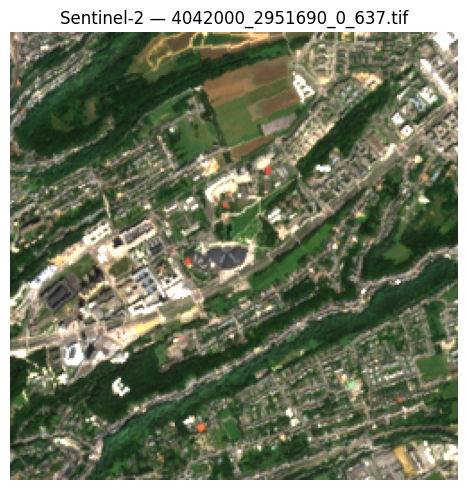

Exercise 5 — Find and display the satellite tile for your city

Goal: Use the filename2bbox.parquet index to find which tile covers your city (from Exercise 4), download it, and display the RGB composite.

Steps:

Build the HTTPS URL to the filename2bbox.parquet file for your NUTS region and year 2024
Read the parquet file with pd.read_parquet()
Extract the city’s EPSG:3035 coordinates from city_point
Loop through the tile bounding boxes to find which one contains your city
Build the full HTTPS URL for the matching tile
Open the tile with rasterio.open(), read the RGB bands, normalize, and display

Hint — Exercise 5

The parquet URL pattern is: https://minio.lab.sspcloud.fr/projet-funathon/2026/project3/data/images/{nuts_code}/{year}/filename2bbox.parquet
pd.read_parquet(url) reads directly from an HTTPS URL (requires pyarrow).
City coordinates: city_point.geometry.iloc[0].x and .y — already in EPSG:3035 from Exercise 4.
Containment check: xmin <= x <= xmax and ymin <= y <= ymax.
The tile URL uses the same base path as the parquet URL, replacing filename2bbox.parquet with the tile filename.
RGB normalization: same technique as Exercise 1 — read bands [4, 3, 2], transpose to (H, W, 3), divide by 98th percentile, clip to [0, 1].

Code template:

import pandas as pd
import rasterio
import numpy as np
import matplotlib.pyplot as plt

# Step 1: Build the parquet URL
year = 2024
parquet_url = ___  # TODO: f"https://minio.lab.sspcloud.fr/.../{nuts_code}/{year}/filename2bbox.parquet"

# Step 2: Read the tile index
tiles = ___  # TODO: pd.read_parquet(...)
print(f"{len(tiles)} tiles available")

# Step 3: Get city coordinates in EPSG:3035
x = ___  # TODO: city_point.geometry.iloc[0].x
y = ___  # TODO: city_point.geometry.iloc[0].y

# Step 4: Find the matching tile
tile_filename = None
for _, row in tiles.iterrows():
    xmin, ymin, xmax, ymax = ___  # TODO: unpack row["bbox"]
    if ___:  # TODO: check xmin <= x <= xmax and ymin <= y <= ymax
        tile_filename = row["filename"]
        break

print(f"Matching tile: {tile_filename}")

# Step 5: Build the full tile URL
tile_url = ___  # TODO

# Step 6: Open, read RGB, normalize and display
with rasterio.open(tile_url) as src:
    rgb_data = ___  # TODO: src.read([4, 3, 2])
    tile_crs = src.crs
    tile_bounds = src.bounds

rgb = np.transpose(rgb_data, (1, 2, 0)).astype(np.float32)
rgb = np.clip(rgb / np.percentile(rgb, 98), 0, 1)

fig, ax = plt.subplots(figsize=(5, 5))
ax.imshow(rgb)
ax.set_title(f"Sentinel-2 — {tile_filename}")
ax.axis("off")
plt.tight_layout()
plt.show()

Solution — Exercise 5

import pandas as pd
import rasterio
import numpy as np
import matplotlib.pyplot as plt

# Step 1: Build the parquet URL
year = 2024
parquet_url = (
    f"https://minio.lab.sspcloud.fr/projet-funathon/2026/"
    f"project3/data/images/{nuts_code}/{year}/filename2bbox.parquet"
)

# Step 2: Read the tile index
tiles = pd.read_parquet(parquet_url)
print(f"{len(tiles)} tiles available")

# Step 3: Get city coordinates in EPSG:3035
x = city_point.geometry.iloc[0].x
y = city_point.geometry.iloc[0].y

# Step 4: Find the matching tile
tile_filename = None
for _, row in tiles.iterrows():
    xmin, ymin, xmax, ymax = row["bbox"]
    if xmin <= x <= xmax and ymin <= y <= ymax:
        tile_filename = row["filename"]
        break

print(f"Matching tile: {tile_filename}")

# Step 5: Build the full tile URL
tile_url = (
    f"https://minio.lab.sspcloud.fr/projet-funathon/2026/"
    f"project3/data/images/{nuts_code}/{year}/{tile_filename}"
)

# Step 6: Open, read RGB, normalize and display
with rasterio.open(tile_url) as src:
    rgb_data = src.read([4, 3, 2])
    tile_crs = src.crs
    tile_bounds = src.bounds

rgb = np.transpose(rgb_data, (1, 2, 0)).astype(np.float32)
rgb = np.clip(rgb / np.percentile(rgb, 98), 0, 1)

fig, ax = plt.subplots(figsize=(5, 5))
ax.imshow(rgb)
ax.set_title(f"Sentinel-2 — {tile_filename}")
ax.axis("off")
plt.tight_layout()
plt.show()

3 Geo-manipulation with GeoPandas

Satellite imagery is inherently geospatial: each pixel corresponds to a precise location on Earth. Before diving into machine-learning pipelines, it is important to know how to manipulate geographic data. GeoPandas extends pandas with geometry support, making CRS transforms, spatial joins, and plotting straightforward.

Vector vs. raster data. So far you have worked with raster data — grids of pixels (satellite images). Geographic boundaries (countries, regions, parcels) are typically stored as vector data — points, lines, and polygons defined by coordinates. GeoPandas lets you work with vector data in a tabular format (like a pandas DataFrame, but with a geometry column).

Tip

Learn more: GeoPandas docs · Shapely docs

3.1 Coordinate Reference Systems

Every raster and vector dataset is tied to a coordinate reference system (CRS) that defines how coordinates map to locations on Earth. CRS mismatch is the single most common source of silent bugs in geospatial work — a join, overlay or distance computation between two layers in different CRS will not raise an error; it will simply return wrong or empty results. The two CRS you will encounter most often in this project are:

CRS	EPSG Code	Units	Use case
WGS 84	4326	Degrees (lat/lon)	GPS, web maps, bounding-box queries
ETRS89-LAEA	3035	Metres	European statistical grids, CLC+ patches

Warning

CRS mismatch is the #1 source of bugs in geospatial projects. If two layers use different CRS, spatial operations (joins, overlays, distance calculations) will produce wrong or empty results. Always check .crs before combining datasets, and use .to_crs() to align them.

Converting between them is a one-liner with GeoPandas:

import geopandas as gpd
from shapely.geometry import box

# Create a GeoDataFrame with the tile extent in EPSG:3035
tile_geom = box(*tile_bounds)
gdf = gpd.GeoDataFrame({"tile": ["LU000"]}, geometry=[tile_geom], crs="EPSG:3035")

print("EPSG:3035 bounds:")
print(gdf.total_bounds)

# Convert to WGS84 (latitude/longitude)
gdf_wgs84 = gdf.to_crs("EPSG:4326")
print("\nEPSG:4326 bounds:")
print(gdf_wgs84.total_bounds)

EPSG:3035 bounds:
[4042000. 2951690. 4044500. 2954190.]

EPSG:4326 bounds:
[ 6.13636681 49.61196423  6.17270527 49.63558621]

Tip

Learn more: epsg.io — search and visualize any coordinate reference system.

3.2 Working with GeoDataFrames

In practice, you can build a GeoDataFrame directly from rasterio metadata — no filename parsing needed:

tile_gdf = gpd.GeoDataFrame(
    {"tile": ["LU000"], "year": [2024]},
    geometry=[box(*tile_bounds)],
    crs=tile_crs,
)
tile_gdf

	tile	year	geometry
0	LU000	2024	POLYGON ((4044500 2951690, 4044500 2954190, 40...

3.3 Overlaying boundaries on images

Combining a raster image with vector boundaries is a common operation. Use imshow with the extent parameter to position the image in coordinate space, then overlay the GeoDataFrame boundary:

fig, ax = plt.subplots(figsize=(6, 6))
extent = [tile_bounds.left, tile_bounds.right, tile_bounds.bottom, tile_bounds.top]
ax.imshow(rgb, extent=extent)
tile_gdf.boundary.plot(ax=ax, color="red", linewidth=2)
ax.set_xlabel("Easting (m)")
ax.set_ylabel("Northing (m)")
ax.set_title("Sentinel-2 tile with boundary overlay (EPSG:3035)")
plt.tight_layout()
plt.show()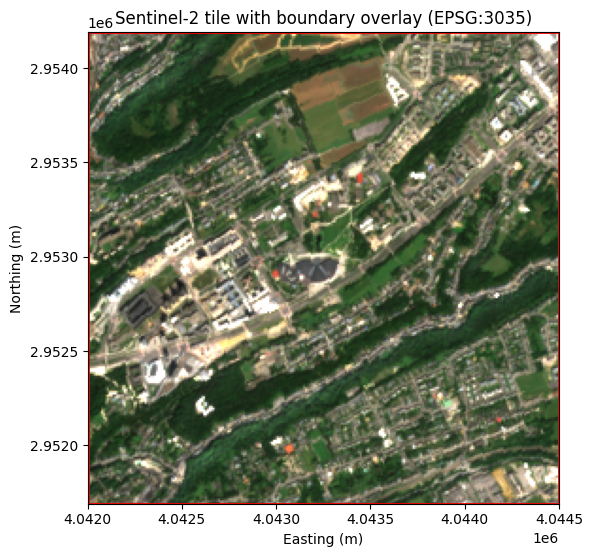

Exercise 6 — Build a GeoDataFrame from tile bounds and convert CRS

Goal: Create a GeoDataFrame from the tile’s bounding box, then convert it from EPSG:3035 to EPSG:4326 (WGS84). Print the bounds in both CRS.

Steps:

Create a shapely.geometry.box from tile_bounds
Build a GeoDataFrame with that geometry and crs="EPSG:3035"
Convert to EPSG:4326 using .to_crs()
Print total_bounds in both CRS

Hint — Exercise 6

box(*tile_bounds) unpacks (left, bottom, right, top) into a rectangular polygon.
gpd.GeoDataFrame({"tile": ["LU000"]}, geometry=[tile_geom], crs="EPSG:3035") creates the GeoDataFrame.
.to_crs("EPSG:4326") reprojects to latitude/longitude.

Code template:

import geopandas as gpd
from shapely.geometry import box

# Step 1: Create a box geometry from tile_bounds
tile_geom = ___  # TODO: box(*tile_bounds)

# Step 2: Build a GeoDataFrame in EPSG:3035
gdf = ___  # TODO: gpd.GeoDataFrame(...)

# Step 3: Convert to WGS84
gdf_wgs84 = ___  # TODO: gdf.to_crs(...)

# Step 4: Print bounds in both CRS
print("EPSG:3035 bounds:", gdf.total_bounds)
print("EPSG:4326 bounds:", gdf_wgs84.total_bounds)

Solution — Exercise 6

import geopandas as gpd
from shapely.geometry import box

tile_geom = box(*tile_bounds)
gdf = gpd.GeoDataFrame({"tile": ["LU000"]}, geometry=[tile_geom], crs="EPSG:3035")
gdf_wgs84 = gdf.to_crs("EPSG:4326")

print("EPSG:3035 bounds:", gdf.total_bounds)
print("EPSG:4326 bounds:", gdf_wgs84.total_bounds)

Exercise 7 — Spatial join with NUTS3 regions

Goal: Identify which NUTS3 region(s) a Sentinel-2 tile intersects using a spatial join, and compute the tile’s area in km².

A spatial join (gpd.sjoin) combines two GeoDataFrames based on the geometric relationship between their features (e.g. intersects, contains, within). This is useful for linking raster tiles to administrative boundaries.

Steps:

Load NUTS3 boundaries from the Eurostat GeoJSON endpoint (EPSG:3035)
Create a GeoDataFrame for the tile (reuse tile_bounds and tile_crs from Exercise 1)
Perform a spatial join with predicate="intersects"
Print the matching NUTS_ID and NUTS_NAME
Compute the tile area in km² (tile_geom.area / 1e6)

Hint — Exercise 7

gpd.read_file(url) can read GeoJSON directly from a URL.
Build the tile GeoDataFrame the same way as in Exercise 6: gpd.GeoDataFrame({"tile": ["LU000"]}, geometry=[box(*tile_bounds)], crs=tile_crs).
gpd.sjoin(left, right, predicate="intersects") returns rows from left enriched with columns from right where geometries intersect.
Since tile_crs is EPSG:3035 (units in metres), tile_geom.area gives square metres — divide by 1 000 000 for km².

Code template:

import geopandas as gpd
from shapely.geometry import box

# Step 7a: Load NUTS3 boundaries (EPSG:3035)
nuts_url = (
    "https://gisco-services.ec.europa.eu/distribution/v2/"
    "nuts/geojson/NUTS_RG_01M_2021_3035_LEVL_3.geojson"
)
nuts = ___  # TODO: gpd.read_file(nuts_url)

# Step 7b: Create a GeoDataFrame for the tile
tile_geom = box(*tile_bounds)
tile_gdf = ___  # TODO: gpd.GeoDataFrame(..., geometry=[tile_geom], crs=tile_crs)

# Step 7c: Spatial join — find which NUTS3 regions the tile intersects
joined = ___  # TODO: gpd.sjoin(tile_gdf, nuts, predicate="intersects")

# Step 7d: Print matching regions
for _, row in joined.iterrows():
    print(f"NUTS_ID: {row['NUTS_ID']}, NUTS_NAME: {row['NUTS_NAME']}")

# Step 7e: Compute tile area in km²
area_km2 = ___  # TODO: tile_geom.area / 1e6
print(f"Tile area: {area_km2:.2f} km²")

Solution — Exercise 7

import geopandas as gpd
from shapely.geometry import box

nuts_url = (
    "https://gisco-services.ec.europa.eu/distribution/v2/"
    "nuts/geojson/NUTS_RG_01M_2021_3035_LEVL_3.geojson"
)
nuts = gpd.read_file(nuts_url)

tile_geom = box(*tile_bounds)
tile_gdf = gpd.GeoDataFrame(
    {"tile": ["LU000"]}, geometry=[tile_geom], crs=tile_crs
)

# Spatial join: for each tile geometry, attach the columns of every NUTS3 region
# whose geometry satisfies the predicate. `predicate="intersects"` keeps any region
# that touches the tile (even partially); alternatives are "within" (tile fully
# inside region) or "contains" (region fully inside tile). A tile straddling a
# border can therefore match several NUTS3 regions — hence the loop below.
joined = gpd.sjoin(tile_gdf, nuts, predicate="intersects")

for _, row in joined.iterrows():
    print(f"NUTS_ID: {row['NUTS_ID']}, NUTS_NAME: {row['NUTS_NAME']}")

# tile_geom is in EPSG:3035 whose unit is the metre, so .area is in m². Divide by
# 1e6 to get km². Computing area on a geographic CRS like EPSG:4326 (degrees) would
# give a meaningless figure — always use a metric projection for measurements.
area_km2 = tile_geom.area / 1e6
print(f"Tile area: {area_km2:.2f} km²")

3.4 Displaying satellite images on a map

3.4.1 Static map with matplotlib

To display the satellite image in geographic coordinates (latitude/longitude), reproject the bounds to WGS84 using rasterio.warp.transform_bounds:

from rasterio.warp import transform_bounds

west, south, east, north = transform_bounds(
    tile_crs, "EPSG:4326", *tile_bounds
)

print(f"WGS84 extent: W={west:.4f}, S={south:.4f}, E={east:.4f}, N={north:.4f}")

fig, ax = plt.subplots(figsize=(6, 6))
ax.imshow(rgb, extent=[west, east, south, north])
ax.set_xlabel("Longitude")
ax.set_ylabel("Latitude")
ax.set_title("Sentinel-2 tile in WGS84 coordinates")
plt.tight_layout()
plt.show()

WGS84 extent: W=6.1364, S=49.6120, E=6.1727, N=49.6356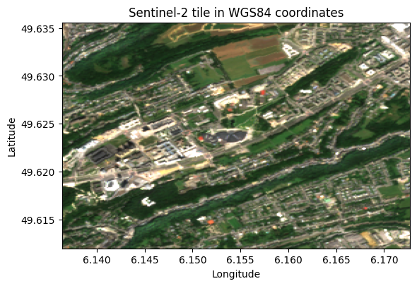

3.4.2 Interactive map with folium

For an interactive web map, use Folium to overlay the satellite image on a basemap.

Important

Reproject the pixels, not just the bounds. Folium and the underlying Leaflet library only render tiles in WGS84 (EPSG:4326, lat/lon). Our Sentinel-2 tile lives in EPSG:3035 (a metric projection used across Europe), so giving Folium the EPSG:3035 pixels with a WGS84 bounding box would stretch the image into the WGS84 rectangle — pixels would shift compared to the basemap, and the distortion grows the farther north you are. To get a correctly aligned overlay we have to resample the pixels themselves onto a WGS84 grid using rasterio.warp.reproject, then hand Folium the warped array. This is the same pipeline used in the inference section.

import folium
import numpy as np
from folium.raster_layers import ImageOverlay
from rasterio.transform import from_bounds
from rasterio.warp import (
    transform_bounds,
    reproject,
    Resampling,
    calculate_default_transform,
)
from rasterio.crs import CRS

dst_crs = CRS.from_epsg(4326)

# rgb_data is the raw (3, H, W) array of R/G/B reflectances in EPSG:3035.
# Derive the source affine transform from the bounds and shape.
h, w = rgb_data.shape[1], rgb_data.shape[2]
src_transform = from_bounds(*tile_bounds, w, h)

# calculate_default_transform picks an output grid in EPSG:4326 that covers the
# same area; reproject() then resamples each band onto that grid.
dst_transform, dst_w, dst_h = calculate_default_transform(
    tile_crs, dst_crs, w, h, *tile_bounds
)

rgb_wgs84_bands = np.zeros((3, dst_h, dst_w), dtype=np.float32)
for i in range(3):
    reproject(
        source=rgb_data[i].astype(np.float32),
        destination=rgb_wgs84_bands[i],
        src_transform=src_transform,
        src_crs=tile_crs,
        dst_transform=dst_transform,
        dst_crs=dst_crs,
        resampling=Resampling.bilinear,  # bilinear for continuous reflectance values
    )

p98 = np.percentile(rgb_wgs84_bands[rgb_wgs84_bands > 0], 98)
rgb_wgs84 = np.clip(np.transpose(rgb_wgs84_bands, (1, 2, 0)) / p98, 0, 1)
# Reprojection from a tilted source produces empty triangular corners. Build an
# alpha channel from "where was there any data?" so those corners stay transparent.
alpha = (rgb_wgs84_bands.max(axis=0) > 0).astype(np.float32)
rgba_wgs84 = np.dstack([rgb_wgs84, alpha])

west, south, east, north = transform_bounds(tile_crs, dst_crs, *tile_bounds)
center_lat = (south + north) / 2
center_lon = (west + east) / 2

m = folium.Map(location=[center_lat, center_lon], zoom_start=14)

ImageOverlay(
    image=rgba_wgs84,
    bounds=[[south, west], [north, east]],
    opacity=0.7,
).add_to(m)

m

Make this Notebook Trusted to load map: File -> Trust Notebook

Tip

Learn more: Folium docs

Exercise 8 — Display a Sentinel-2 tile on an interactive folium map

Goal: Reproject the RGB image to WGS84 and display it on an interactive folium map. Because Folium only renders EPSG:4326 tiles, you must warp the pixels — not just the bounding box — onto a WGS84 grid.

Steps:

Use calculate_default_transform() to compute the output grid in EPSG:4326
Call reproject() once per RGB band with Resampling.bilinear to warp the pixels onto that grid
Normalize the warped bands to [0, 1] and build an alpha channel from the data mask (transparent corners)
Use transform_bounds() to get the WGS84 (west, south, east, north) of the tile
Create a folium.Map centred on the tile and add an ImageOverlay with the warped RGBA array

Hint — Exercise 8

calculate_default_transform(tile_crs, dst_crs, w, h, *tile_bounds) returns the WGS84 grid that covers the same area.
Loop over the 3 RGB bands and call reproject(...) per band, writing into the corresponding slice of rgb_wgs84_bands (shape == (3, dst_h, dst_w)).
Use Resampling.bilinear for reflectance (continuous values). Resampling.nearest is for categorical rasters like labels.
alpha = (rgb_wgs84_bands.max(axis=0) > 0).astype(np.float32) turns the empty triangular corners (from the rotated source) into transparent pixels.
transform_bounds(tile_crs, "EPSG:4326", *tile_bounds) returns (west, south, east, north) in degrees.
ImageOverlay(image=rgba_wgs84, bounds=[[south, west], [north, east]], opacity=0.7).add_to(m) overlays the warped image.

Code template:

import folium
import numpy as np
from folium.raster_layers import ImageOverlay
from rasterio.transform import from_bounds
from rasterio.warp import (
    transform_bounds,
    reproject,
    Resampling,
    calculate_default_transform,
)
from rasterio.crs import CRS

dst_crs = CRS.from_epsg(4326)

# Step 1: Compute the WGS84 output grid
h, w = rgb_data.shape[1], rgb_data.shape[2]
src_transform = from_bounds(*tile_bounds, w, h)
dst_transform, dst_w, dst_h = ___  # TODO: calculate_default_transform(...)

# Step 2: Reproject each band onto that grid
rgb_wgs84_bands = np.zeros((3, dst_h, dst_w), dtype=np.float32)
for i in range(3):
    reproject(
        source=rgb_data[i].astype(np.float32),
        destination=rgb_wgs84_bands[i],
        src_transform=src_transform,
        src_crs=___,         # TODO: source CRS
        dst_transform=dst_transform,
        dst_crs=___,         # TODO: destination CRS
        resampling=___,      # TODO: Resampling.bilinear (continuous values)
    )

# Step 3: Normalize + alpha channel for transparent corners
p98 = np.percentile(rgb_wgs84_bands[rgb_wgs84_bands > 0], 98)
rgb_wgs84 = np.clip(np.transpose(rgb_wgs84_bands, (1, 2, 0)) / p98, 0, 1)
alpha = ___  # TODO: (rgb_wgs84_bands.max(axis=0) > 0).astype(np.float32)
rgba_wgs84 = np.dstack([rgb_wgs84, alpha])

# Step 4: Reproject the bounds and pick a centre
west, south, east, north = ___  # TODO: transform_bounds(...)
center_lat = ___  # TODO
center_lon = ___  # TODO

# Step 5: Build the folium map
m = ___  # TODO: folium.Map(...)
___  # TODO: ImageOverlay(image=rgba_wgs84, ...).add_to(m)

m

Solution — Exercise 8

import folium
import numpy as np
from folium.raster_layers import ImageOverlay
from rasterio.transform import from_bounds
from rasterio.warp import (
    transform_bounds,
    reproject,
    Resampling,
    calculate_default_transform,
)
from rasterio.crs import CRS

dst_crs = CRS.from_epsg(4326)

# Step 1: Compute the WGS84 output grid that covers the tile
h, w = rgb_data.shape[1], rgb_data.shape[2]
src_transform = from_bounds(*tile_bounds, w, h)
dst_transform, dst_w, dst_h = calculate_default_transform(
    tile_crs, dst_crs, w, h, *tile_bounds
)

# Step 2: Reproject each RGB band onto that grid
rgb_wgs84_bands = np.zeros((3, dst_h, dst_w), dtype=np.float32)
for i in range(3):
    reproject(
        source=rgb_data[i].astype(np.float32),
        destination=rgb_wgs84_bands[i],
        src_transform=src_transform,
        src_crs=tile_crs,
        dst_transform=dst_transform,
        dst_crs=dst_crs,
        resampling=Resampling.bilinear,
    )

# Step 3: Normalize to [0, 1] and build the alpha channel
p98 = np.percentile(rgb_wgs84_bands[rgb_wgs84_bands > 0], 98)
rgb_wgs84 = np.clip(np.transpose(rgb_wgs84_bands, (1, 2, 0)) / p98, 0, 1)
alpha = (rgb_wgs84_bands.max(axis=0) > 0).astype(np.float32)
rgba_wgs84 = np.dstack([rgb_wgs84, alpha])

# Step 4: Reproject the bounds and centre the map
west, south, east, north = transform_bounds(tile_crs, dst_crs, *tile_bounds)
center_lat = (south + north) / 2
center_lon = (west + east) / 2

# Step 5: Build the map
m = folium.Map(location=[center_lat, center_lon], zoom_start=14)
ImageOverlay(
    image=rgba_wgs84,
    bounds=[[south, west], [north, east]],
    opacity=0.7,
).add_to(m)

m

4 CLC+ Backbone Labels — Land-Cover Ground Truth

In supervised machine learning, you need pairs of inputs and labels to train a model. The inputs are the Sentinel-2 satellite images; the labels are provided by CLC+ Backbone, a high-resolution land-cover product from the Copernicus Land Monitoring Service.

What does CLC stand for? CLC is short for CORINE Land Cover (Coordination of Information on the Environment — Land Cover), the European reference inventory of land cover and land use. First produced in 1990 and updated roughly every six years, it has long been the standard product for tracking land-cover change across Europe. CLC+ Backbone is the next-generation evolution of this programme: instead of the original 44 hierarchical classes mapped at 100 m resolution from manually delineated polygons, it delivers a pixel-level raster at 10 m resolution with a simplified set of 10 land-cover classes, derived automatically from Sentinel-2 imagery — which makes it directly suitable as ground truth for a deep-learning segmentation model.

CLC+ Backbone provides pixel-level land-cover classification across Europe at 10 m resolution, making it an ideal ground-truth dataset for training and evaluating segmentation models. The labels are temporally aligned with the satellite imagery (same year), ensuring that the land-cover classification corresponds to what the satellite actually observed.

Why 2021? CLC+ Backbone’s most recent public release at the time of writing is the 2021 edition, so that’s the year we use for labels. Each label is paired with a Sentinel-2 image from the same year — land cover actually changes between years (new construction, deforestation, crop rotation), and mismatched pairs would teach the model to predict yesterday’s ground truth for today’s image. The 2024 Sentinel-2 imagery you saw in the earlier exercises is kept for Chapter 3, where we run the trained model on new images that have no label — which is the whole point of training a model in the first place.

4.1 Land-cover classes

CLC+ Backbone uses 10 land-cover classes:

Class ID	Name	Description
1	Sealed	Buildings, roads, paved surfaces
2	Woody – needle leaved	Coniferous forests
3	Woody – broadleaved deciduous	Deciduous forests
4	Woody – broadleaved evergreen	Evergreen broadleaved forests
5	Low-growing woody plants	Bushes, shrubs
6	Permanent herbaceous	Grasslands, meadows
7	Periodically herbaceous	Croplands
8	Lichens and mosses	Natural low vegetation
9	Non- and sparsely-vegetated	Bare soil, rock
10	Water	Rivers, lakes, sea

Note

Nodata values. The raw CLC+ raster may contain values 254 and 255, which represent “unclassified” and “nodata” respectively. The tiff_to_numpy() utility maps these to 0 so they do not interfere with the 1–10 class range.

4.2 How labels are stored on S3

Pre-processed CLC+ Backbone labels are publicly available on the SSP Cloud object storage, alongside the satellite images. Each label is a 2D NumPy array (.npy file) of shape (250, 250) with uint8 values representing land-cover class IDs (1–10, with 0 for nodata).

The HTTPS URL follows this pattern:

https://minio.lab.sspcloud.fr/projet-funathon/2026/project3/data/labels/{NUTS}/{year}/{patch_id}.npy

The label and image paths mirror each other — to find the label for a given image, replace images with labels and .tif with .npy:

.../data/images/{NUTS}/{year}/{patch_id}.tif   ← satellite image (GeoTIFF)
.../data/labels/{NUTS}/{year}/{patch_id}.npy   ← land-cover label (NumPy)

The {patch_id} encodes {xmin}_{ymin}_{idx}_{id} in EPSG:3035 metres and is identical between images and labels.

Note

Loading .npy from a URL. Unlike GeoTIFF files (which rasterio can open directly from a URL), .npy files must be fetched into memory first. The three-step idiom is:

urllib.request.urlopen(url) — opens the remote URL and lets you call .read() on it to pull down the raw bytes.
io.BytesIO(response.read()) — wraps those raw bytes in an in-memory file-like object. This step exists because np.load expects something it can call .read() on (a file handle or an equivalent stream), not a plain bytes value.
np.load(...) — parses that stream back into a NumPy array.

.npy files contain no embedded CRS or bounds metadata — the spatial information is encoded in the filename and matches the corresponding image tile.

Tip

Learn more: CLC+ Backbone product page · Copernicus Land Monitoring Service

4.3 Loading and displaying a label

Let’s load a CLC+ label from S3 and display it next to its matching satellite image. The three-step pattern for loading a .npy file over HTTPS is: open the URL → read into a bytes buffer → load with NumPy.

import urllib.request
import io
import numpy as np

# Label URL for a LU000 patch, year 2021
label_url = (
    "https://minio.lab.sspcloud.fr/projet-funathon/2026/"
    "project3/data/labels/LU000/"
    "2021/4042000_2951690_0_637.npy"
)

with urllib.request.urlopen(label_url) as response:
    label_array = np.load(io.BytesIO(response.read()))

print(f"Label shape: {label_array.shape}")
print(f"Data type:   {label_array.dtype}")
print(f"Classes:     {np.unique(label_array)}")

Label shape: (250, 250)
Data type:   uint8
Classes:     [ 1  2  3  5  6  7  9 10]

We can visualise the label using a custom colormap that assigns a colour to each of the 10 land-cover classes:

import rasterio
import matplotlib.pyplot as plt
from matplotlib.colors import ListedColormap
from matplotlib.patches import Patch

# CLC+ class names and colours
classes = [
    ("Sealed (1)", "#FF0100"),
    ("Woody -- needle leaved trees (2)", "#238B23"),
    ("Woody -- Broadleaved deciduous trees (3)", "#80FF00"),
    ("Woody -- Broadleaved evergreen trees (4)", "#00FF00"),
    ("Low-growing woody plants (bushes, shrubs) (5)", "#804000"),
    ("Permanent herbaceous (6)", "#CCF24E"),
    ("Periodically herbaceous (7)", "#FEFF80"),
    ("Lichens and mosses (8)", "#FF81FF"),
    ("Non- and sparsely-vegetated (9)", "#BFBFBF"),
    ("Water (10)", "#0080FF"),
]
cmap = ListedColormap([color for _, color in classes])

# Load the matching satellite image
image_url = (
    "https://minio.lab.sspcloud.fr/projet-funathon/2026/"
    "project3/data/images/LU000/"
    "2021/4042000_2951690_0_637.tif"
)
with rasterio.open(image_url) as src:
    rgb_data = src.read([4, 3, 2])

rgb = np.transpose(rgb_data, (1, 2, 0)).astype(np.float32)
rgb = np.clip(rgb / np.percentile(rgb, 98), 0, 1)

# Side-by-side plot
fig, axes = plt.subplots(1, 2, figsize=(12, 5))

axes[0].imshow(rgb)
axes[0].set_title("Sentinel-2 RGB")
axes[0].axis("off")

axes[1].imshow(label_array, cmap=cmap, vmin=1, vmax=10)
axes[1].set_title("CLC+ Backbone label")
axes[1].axis("off")

legend_elements = [
    Patch(facecolor=color, edgecolor="black", label=label)
    for label, color in classes
]
fig.legend(
    handles=legend_elements,
    loc="center right",
    bbox_to_anchor=(1.30, 0.5),
    frameon=True,
)
plt.tight_layout()
plt.show()

4.4 Label–image alignment — this is the training target

What you just displayed is exactly what the model is trained on. The RGB image on the left is the input; the coloured mask on the right is the target. The entire goal of the segmentation model is this: given a new Sentinel-2 tile that the model has never seen, produce a mask of the same shape with the correct class at every pixel.

This only works because the images and labels are spatially aligned by construction: they share the same CRS (EPSG:3035) and bounding box, and use identical filenames ({xmin}_{ymin}_{idx}_{id}). Pixel (i, j) in the label therefore refers to the same 10 m patch of ground as pixel (i, j) in the image — always. A large collection of such (image, label) pairs is exactly what Chapter 2 feeds to the model during training.

Exercise 9 — Load a CLC+ label from S3

Goal: Load the CLC+ Backbone label for a patch of your choice from S3 over HTTPS, and display it with the land-cover colormap.

Steps:

Choose a NUTS region, year (2021), and patch ID (you can reuse the tile found in Exercise 5, replacing .tif with .npy)
Build the HTTPS URL following the label path pattern
Fetch the .npy file using urllib.request.urlopen() and load it with np.load(io.BytesIO(...))
Print the array shape and unique class values
Display the label using imshow() with the CLC+ colormap (vmin=1, vmax=10)

Hint — Exercise 9

The label URL pattern is: https://minio.lab.sspcloud.fr/projet-funathon/2026/project3/data/labels/{NUTS}/{year}/{patch_id}.npy
Use urllib.request.urlopen(url) as a context manager, then np.load(io.BytesIO(response.read())) to load the array.
np.unique(my_label) returns the distinct class IDs present in the tile.
Set vmin=1, vmax=10 in imshow() so the colormap maps correctly to the 10 classes.

Code template:

import urllib.request
import io
import numpy as np
import matplotlib.pyplot as plt
from matplotlib.colors import ListedColormap

# Step 1: Choose your tile
nuts_code = ___  # TODO: e.g. "LU000"
year = ___        # TODO: e.g. 2021
patch_id = ___    # TODO: e.g. "4042000_2951690_0_637"

# Step 2: Build the label URL
label_url = ___  # TODO: f"https://minio.lab.sspcloud.fr/projet-funathon/2026/project3/data/labels/{nuts_code}/{year}/{patch_id}.npy"

# Step 3: Load the label
with urllib.request.urlopen(label_url) as response:
    my_label = ___  # TODO: np.load(io.BytesIO(response.read()))

# Step 4: Inspect
print(f"Shape: {___}")   # TODO
print(f"Classes: {___}")  # TODO

# Step 5: Display with CLC+ colormap
cmap = ListedColormap([
    "#FF0100", "#238B23", "#80FF00", "#00FF00", "#804000",
    "#CCF24E", "#FEFF80", "#FF81FF", "#BFBFBF", "#0080FF",
])

fig, ax = plt.subplots(figsize=(5, 5))
___  # TODO: ax.imshow(my_label, cmap=cmap, vmin=1, vmax=10)
ax.set_title(f"CLC+ label — {nuts_code}/{year}/{patch_id}")
ax.axis("off")
plt.show()

Solution — Exercise 9

import urllib.request
import io
import numpy as np
import matplotlib.pyplot as plt
from matplotlib.colors import ListedColormap

nuts_code = "LU000"
year = 2021
patch_id = "4042000_2951690_0_637"

label_url = f"https://minio.lab.sspcloud.fr/projet-funathon/2026/project3/data/labels/{nuts_code}/{year}/{patch_id}.npy"

with urllib.request.urlopen(label_url) as response:
    my_label = np.load(io.BytesIO(response.read()))

print(f"Shape: {my_label.shape}")
print(f"Classes: {np.unique(my_label)}")

cmap = ListedColormap(
    [
        "#FF0100",
        "#238B23",
        "#80FF00",
        "#00FF00",
        "#804000",
        "#CCF24E",
        "#FEFF80",
        "#FF81FF",
        "#BFBFBF",
        "#0080FF",
    ]
)

fig, ax = plt.subplots(figsize=(5, 5))
ax.imshow(my_label, cmap=cmap, vmin=1, vmax=10)
ax.set_title(f"CLC+ label — {nuts_code}/{year}/{patch_id}")
ax.axis("off")
plt.show()

Before training any model, it is good practice to inspect the training data visually: do the labels really correspond to what the imagery shows? Overlaying the CLC+ classification on top of the Sentinel-2 RGB tile makes mis-aligned, mis-classified or stale labels obvious in a few seconds of scrolling — much faster than computing summary statistics. An interactive map with toggleable layers lets you flip the labels on and off to check the boundary lines class by class.

Exercise 10 — Overlay the satellite image and CLC+ label on an interactive map

Goal: Create an interactive folium map displaying both the Sentinel-2 RGB composite and the CLC+ land-cover label as toggleable overlays. Both rasters live in EPSG:3035 and must be reprojected to WGS84 — pixels and all — before Folium can render them correctly (same reasoning as Exercise 8).

Steps:

Load the satellite image for LU000/2021 with rasterio and read RGB bands (4, 3, 2)
Load the matching CLC+ label from S3
Reproject the RGB bands to WGS84 with Resampling.bilinear (continuous reflectance) and the integer label with Resampling.nearest (categorical — bilinear would invent non-existent class IDs)
Normalize the warped RGB, build an alpha channel for the empty corners, and apply a colour lookup table to the warped label
Reproject the tile bounds with transform_bounds(), create a folium.Map, and add the two ImageOverlay layers
Add a folium.LayerControl() so layers can be toggled on and off

Hint — Exercise 10

Resampling.bilinear for the RGB bands; Resampling.nearest for the label (do not average integer class IDs).
Use the same dst_transform / dst_w / dst_h for both rasters so the two layers stay pixel-aligned.
Apply the colour LUT after warping (color_lut[label_wgs84]), so the LUT maps integer class IDs and the alpha channel of class 0 stays exact.
to_rgba("#FF0100", alpha=0.7) returns an RGBA tuple with values in [0, 1].
transform_bounds(src_crs, "EPSG:4326", left, bottom, right, top) returns (west, south, east, north) in WGS84.
ImageOverlay(image=array, bounds=[[south, west], [north, east]], name="Layer Name") — the name parameter is what appears in LayerControl.
folium.LayerControl().add_to(m) adds a toggle widget to switch layers on and off.

Code template:

import numpy as np
import urllib.request
import io
import rasterio
import folium
from rasterio.transform import from_bounds
from rasterio.warp import (
    transform_bounds,
    reproject,
    Resampling,
    calculate_default_transform,
)
from rasterio.crs import CRS
from matplotlib.colors import to_rgba

# --- Given: class colours (same as the colormap above) ---
classes = [
    ("Sealed (1)", "#FF0100"),
    ("Woody -- needle leaved trees (2)", "#238B23"),
    ("Woody -- Broadleaved deciduous trees (3)", "#80FF00"),
    ("Woody -- Broadleaved evergreen trees (4)", "#00FF00"),
    ("Low-growing woody plants (bushes, shrubs) (5)", "#804000"),
    ("Permanent herbaceous (6)", "#CCF24E"),
    ("Periodically herbaceous (7)", "#FEFF80"),
    ("Lichens and mosses (8)", "#FF81FF"),
    ("Non- and sparsely-vegetated (9)", "#BFBFBF"),
    ("Water (10)", "#0080FF"),
]

# Step 1: Load satellite image (raw bands, no normalization yet)
image_url = (
    "https://minio.lab.sspcloud.fr/projet-funathon/2026/"
    "project3/data/images/LU000/"
    "2021/4017000_2974190_0_402.tif"
)
with rasterio.open(image_url) as src:
    rgb_data = src.read([4, 3, 2])
    bounds_3035 = src.bounds
    crs = src.crs

# Step 2: Load the matching label
label_url = (
    "https://minio.lab.sspcloud.fr/projet-funathon/2026/"
    "project3/data/labels/LU000/"
    "2021/4017000_2974190_0_402.npy"
)
with urllib.request.urlopen(label_url) as response:
    label = np.load(io.BytesIO(response.read()))

# Step 3: Reproject both rasters onto a common WGS84 grid
dst_crs = CRS.from_epsg(4326)
h, w = rgb_data.shape[1], rgb_data.shape[2]
src_transform = from_bounds(*bounds_3035, w, h)
dst_transform, dst_w, dst_h = calculate_default_transform(
    crs, dst_crs, w, h, *bounds_3035
)

rgb_wgs84_bands = np.zeros((3, dst_h, dst_w), dtype=np.float32)
for i in range(3):
    reproject(
        source=rgb_data[i].astype(np.float32),
        destination=rgb_wgs84_bands[i],
        src_transform=src_transform,
        src_crs=crs,
        dst_transform=dst_transform,
        dst_crs=dst_crs,
        resampling=___,  # TODO: bilinear for continuous reflectance
    )

label_wgs84 = np.zeros((dst_h, dst_w), dtype=label.dtype)
reproject(
    source=label,
    destination=label_wgs84,
    src_transform=src_transform,
    src_crs=crs,
    dst_transform=dst_transform,
    dst_crs=dst_crs,
    resampling=___,  # TODO: nearest for categorical class IDs
)

# Step 4: Build the RGB overlay (normalize + alpha) and the label RGBA (colour LUT)
p98 = np.percentile(rgb_wgs84_bands[rgb_wgs84_bands > 0], 98)
rgb_overlay = np.clip(np.transpose(rgb_wgs84_bands, (1, 2, 0)) / p98, 0, 1)
alpha = (rgb_wgs84_bands.max(axis=0) > 0).astype(np.float32)
rgba_overlay = np.dstack([rgb_overlay, alpha])

color_lut = np.zeros((11, 4), dtype=np.float32)
color_lut[0] = ___  # TODO: [0, 0, 0, 0]  (fully transparent for nodata)
for i, (_, hex_color) in enumerate(classes, start=1):
    color_lut[i] = ___  # TODO: list(to_rgba(hex_color, alpha=0.7))

label_rgba = ___  # TODO: color_lut[label_wgs84]

# Step 5: Reproject bounds and build the map
west, south, east, north = ___  # TODO: transform_bounds(crs, "EPSG:4326", *bounds_3035)

center_lat = ___  # TODO: (south + north) / 2
center_lon = ___  # TODO: (west + east) / 2

m = ___  # TODO: folium.Map(location=[center_lat, center_lon], zoom_start=15)

___  # TODO: folium.raster_layers.ImageOverlay(image=rgba_overlay, bounds=[[south, west], [north, east]], name="Sentinel-2 RGB").add_to(m)
___  # TODO: folium.raster_layers.ImageOverlay(image=label_rgba, bounds=[[south, west], [north, east]], name="CLC+ Label", opacity=0.8).add_to(m)

# Step 6: Layer control
___  # TODO: folium.LayerControl().add_to(m)

m

Solution — Exercise 10

import numpy as np
import urllib.request
import io
import rasterio
import folium
from rasterio.transform import from_bounds
from rasterio.warp import (
    transform_bounds,
    reproject,
    Resampling,
    calculate_default_transform,
)
from rasterio.crs import CRS
from matplotlib.colors import to_rgba

classes = [
    ("Sealed (1)", "#FF0100"),
    ("Woody -- needle leaved trees (2)", "#238B23"),
    ("Woody -- Broadleaved deciduous trees (3)", "#80FF00"),
    ("Woody -- Broadleaved evergreen trees (4)", "#00FF00"),
    ("Low-growing woody plants (bushes, shrubs) (5)", "#804000"),
    ("Permanent herbaceous (6)", "#CCF24E"),
    ("Periodically herbaceous (7)", "#FEFF80"),
    ("Lichens and mosses (8)", "#FF81FF"),
    ("Non- and sparsely-vegetated (9)", "#BFBFBF"),
    ("Water (10)", "#0080FF"),
]

# Step 1: Load satellite image
image_url = (
    "https://minio.lab.sspcloud.fr/projet-funathon/2026/"
    "project3/data/images/LU000/"
    "2021/4017000_2974190_0_402.tif"
)
with rasterio.open(image_url) as src:
    rgb_data = src.read([4, 3, 2])
    bounds_3035 = src.bounds
    crs = src.crs

# Step 2: Load the matching label
label_url = (
    "https://minio.lab.sspcloud.fr/projet-funathon/2026/"
    "project3/data/labels/LU000/"
    "2021/4017000_2974190_0_402.npy"
)
with urllib.request.urlopen(label_url) as response:
    label = np.load(io.BytesIO(response.read()))

# Step 3: Reproject both rasters onto a common WGS84 grid.
# RGB → Resampling.bilinear (continuous values); label → Resampling.nearest
# (categorical: averaging integer class IDs would invent classes that don't exist).
dst_crs = CRS.from_epsg(4326)
h, w = rgb_data.shape[1], rgb_data.shape[2]
src_transform = from_bounds(*bounds_3035, w, h)
dst_transform, dst_w, dst_h = calculate_default_transform(
    crs, dst_crs, w, h, *bounds_3035
)

rgb_wgs84_bands = np.zeros((3, dst_h, dst_w), dtype=np.float32)
for i in range(3):
    reproject(
        source=rgb_data[i].astype(np.float32),
        destination=rgb_wgs84_bands[i],
        src_transform=src_transform,
        src_crs=crs,
        dst_transform=dst_transform,
        dst_crs=dst_crs,
        resampling=Resampling.bilinear,
    )

label_wgs84 = np.zeros((dst_h, dst_w), dtype=label.dtype)
reproject(
    source=label,
    destination=label_wgs84,
    src_transform=src_transform,
    src_crs=crs,
    dst_transform=dst_transform,
    dst_crs=dst_crs,
    resampling=Resampling.nearest,
)

# Step 4: Build RGB overlay (normalize + alpha for empty corners) and label RGBA.
p98 = np.percentile(rgb_wgs84_bands[rgb_wgs84_bands > 0], 98)
rgb_overlay = np.clip(np.transpose(rgb_wgs84_bands, (1, 2, 0)) / p98, 0, 1)
alpha = (rgb_wgs84_bands.max(axis=0) > 0).astype(np.float32)
rgba_overlay = np.dstack([rgb_overlay, alpha])

color_lut = np.zeros((11, 4), dtype=np.float32)
color_lut[0] = [0, 0, 0, 0]
for i, (_, hex_color) in enumerate(classes, start=1):
    color_lut[i] = list(to_rgba(hex_color, alpha=0.7))

label_rgba = color_lut[label_wgs84]

# Step 5: Reproject bounds and build the map
west, south, east, north = transform_bounds(crs, "EPSG:4326", *bounds_3035)

center_lat = (south + north) / 2
center_lon = (west + east) / 2

m = folium.Map(location=[center_lat, center_lon], zoom_start=15)

folium.raster_layers.ImageOverlay(
    image=rgba_overlay,
    bounds=[[south, west], [north, east]],
    name="Sentinel-2 RGB",
).add_to(m)

folium.raster_layers.ImageOverlay(
    image=label_rgba,
    bounds=[[south, west], [north, east]],
    name="CLC+ Label",
    opacity=0.8,
).add_to(m)

# Step 6: Layer control
folium.LayerControl().add_to(m)

m

5 Summary

In this chapter you built the full data pipeline that feeds a land-cover segmentation model:

Step	What you did	Key tools
Load & explore imagery	Opened a Sentinel-2 GeoTIFF, read spectral bands, and inspected raster metadata	`rasterio`
Visualise composites	Displayed true-colour and false-colour composites; computed NDVI	`numpy`, `matplotlib`
Geospatial manipulation	Worked with CRS, built geometries, performed spatial joins, and plotted interactive maps	`geopandas`, `shapely`, `folium`
Navigate the tile index	Geocoded a city with Nominatim, resolved its NUTS3 region, and found the covering tile with the `filename2bbox.parquet` index	`requests`, `geopandas`
Load CLC+ labels	Downloaded pre-processed land-cover labels from S3 and paired them pixel-for-pixel with satellite images	`numpy`, `urllib`
(Optional) Acquire new data	Downloaded CLC+ labels from the Copernicus ImageServer; queried and downloaded Sentinel-2 imagery from the Sentinel Hub and OData APIs	`requests`, `rasterio.io.MemoryFile`

5.1 What’s next?

You now have aligned image / label pairs — the raw material for supervised learning. You can continue with either:

Model Explanation — walk through the SegFormer architecture used for segmentation.
Model Training (optional) — train a SegFormer segmentation model on the Sentinel-2 / CLC+ pairs you assembled here.
Inference — run a pre-trained model on new tiles, to map land cover predictions on newer images.

If you’re curious about where the pre-processed patches come from and how you would build them for a different region, the Appendix walks through the full download pipeline from the original Copernicus APIs.

Appendix — Acquiring data from source APIs

Acquiring CLC+ Labels from APIs

Optional — Click to expand

This section shows how to download CLC+ Backbone labels directly from the Copernicus Land Monitoring Service REST API and prepare them for the training pipeline. It is not needed for the rest of the sections — the pre-processed labels on S3 are sufficient.

5.1.1 Downloading from the Copernicus Land Monitoring Service ImageServer

Labels can be downloaded directly from the Copernicus Land Monitoring Service using the ArcGIS ImageServer exportImage endpoint. No authentication is required. The bounding box must match the satellite tile extent exactly to ensure pixel-level alignment.

import requests
import numpy as np
import rasterio
from rasterio.io import MemoryFile

year = 2021
export_url = (
    f"https://copernicus.discomap.eea.europa.eu/arcgis/rest/services/CLC_plus/"
    f"CLMS_CLCplus_RASTER_{year}_010m_eu/ImageServer/exportImage"
)

bbox = [3649890, 2331750, 3652390, 2334250]
xmin, ymin, xmax, ymax = bbox
resolution = 10  # 1 pixel = 10 m
size_x = int((xmax - xmin) / resolution)
size_y = int((ymax - ymin) / resolution)

params = {
    "f": "image",
    "bbox": f"{xmin},{ymin},{xmax},{ymax}",
    "bboxSR": "3035",
    "imageSR": "3035",
    "size": f"{size_x},{size_y}",
    "format": "tiff",
}

response = requests.get(export_url, params=params)
response.raise_for_status()

with MemoryFile(response.content) as memfile:
    with memfile.open() as src:
        label_array = src.read(1)  # single band, shape (H, W)

# Map nodata values to 0 (254 = unclassified, 255 = nodata)
label_array[(label_array == 254) | (label_array == 255)] = 0
print(f"Label shape: {label_array.shape}, classes: {np.unique(label_array)}")

Exercise 11 (optional) — Download a CLC+ label from the ImageServer API

Goal: Query the Copernicus Land Monitoring Service ImageServer directly to download the CLC+ Backbone label matching a Sentinel-2 patch, and convert it to a NumPy array.

Steps:

Define the bounding box [3649890, 2331750, 3652390, 2334250] (EPSG:3035) and compute pixel dimensions (1 px = 10 m)
Build the exportImage URL for year=2021
Send a GET request with the required parameters and raise on HTTP errors
Load the TIFF response in-memory with MemoryFile(response.content) and read band 1
Map nodata values 254 and 255 to 0

import requests
import numpy as np
import rasterio
from rasterio.io import MemoryFile

# Step 1: Define bounding box and compute pixel dimensions
year = 2021
bbox = [3649890, 2331750, 3652390, 2334250]
xmin, ymin, xmax, ymax = bbox
resolution = 10  # 1 pixel = 10 m
size_x = ___  # TODO: int((xmax - xmin) / resolution)
size_y = ___  # TODO: int((ymax - ymin) / resolution)

# Step 2: Build the exportImage URL
export_url = ___  # TODO: f"https://copernicus.discomap.eea.europa.eu/arcgis/rest/services/CLC_plus/CLMS_CLCplus_RASTER_{year}_010m_eu/ImageServer/exportImage"

# Step 3: Send the request
params = {
    "f": "image",
    "bbox": f"{xmin},{ymin},{xmax},{ymax}",
    "bboxSR": "3035",
    "imageSR": "3035",
    "size": f"{size_x},{size_y}",
    "format": "tiff",
}
response = ___  # TODO: requests.get(export_url, params=params)
___  # TODO: response.raise_for_status()

# Step 4: Load TIFF from memory and read band 1
with MemoryFile(___) as memfile:  # TODO: response.content
    with memfile.open() as src:
        img_array = ___  # TODO: src.read(1)

# Step 5: Map nodata values to 0
img_array[___] = 0  # TODO: (img_array == 254) | (img_array == 255)

Hint — Exercise 11

The ImageServer URL pattern: https://copernicus.discomap.eea.europa.eu/arcgis/rest/services/CLC_plus/CLMS_CLCplus_RASTER_{year}_010m_eu/ImageServer/exportImage
bboxSR and imageSR both set to "3035" keep the data in EPSG:3035 (metres).
size must match the bbox extent: size_x = int((xmax - xmin) / 10), size_y = int((ymax - ymin) / 10).
MemoryFile(response.content) wraps the raw bytes so rasterio can open the TIFF without writing to disk.
src.read(1) reads band 1 as a 2D NumPy array of shape (H, W).

Solution — Exercise 11

import requests
import numpy as np
import rasterio
from rasterio.io import MemoryFile

year = 2021
bbox = [3649890, 2331750, 3652390, 2334250]
xmin, ymin, xmax, ymax = bbox
resolution = 10
size_x = int((xmax - xmin) / resolution)
size_y = int((ymax - ymin) / resolution)

export_url = (
    f"https://copernicus.discomap.eea.europa.eu/arcgis/rest/services/CLC_plus/"
    f"CLMS_CLCplus_RASTER_{year}_010m_eu/ImageServer/exportImage"
)

params = {
    "f": "image",
    "bbox": f"{xmin},{ymin},{xmax},{ymax}",
    "bboxSR": "3035",
    "imageSR": "3035",
    "size": f"{size_x},{size_y}",
    "format": "tiff",
}

response = requests.get(export_url, params=params)
response.raise_for_status()

with MemoryFile(response.content) as memfile:
    with memfile.open() as src:
        img_array = src.read(1)

img_array[(img_array == 254) | (img_array == 255)] = 0

5.1.2 Uploading labels to S3

The training pipeline in section 2 expects labels as NumPy .npy files stored on S3, following a specific path convention:

# Satellite image
s3://projet-funathon/2026/project3/data/images/{NUTS}/{year}/{patch_id}.tif

# Corresponding label
s3://projet-funathon/2026/project3/data/labels/{NUTS}/{year}/{patch_id}.npy

Exercise 12 (optional) — Save the label as .npy and upload to S3

Goal: Save the label array from Exercise 11 as a .npy file and upload it to S3 in the path expected by the training pipeline.

Steps:

Save img_array locally as a .npy file using np.save()
Initialise an S3FileSystem with get_file_system() (from utils)
Build the S3 destination path matching the training pipeline convention
Upload the local file with fs.put()
Verify the upload by listing the S3 directory with fs.ls()

import numpy as np
from src.utils import get_file_system

# Step 1: Save the label array locally as .npy
local_path = "3649890_2331750_0_937.npy"
___  # TODO: np.save(local_path, img_array)

# Step 2: Initialise the S3 filesystem
fs = ___  # TODO: get_file_system()

# Step 3: Build the S3 destination path
s3_path = ___  # TODO: "projet-funathon/2026/project3/data/images/LU000/2024/250/3649890_2331750_0_937.npy"

# Step 4: Upload to S3
___  # TODO: fs.put(local_path, s3_path)

# Step 5: Verify the upload
print(fs.ls(___))  # TODO: S3 directory path (without filename)

Hint — Exercise 12

np.save("file.npy", array) saves a NumPy array to disk.
get_file_system() returns an s3fs.S3FileSystem configured with the SSP Cloud credentials.
The S3 path must not include the s3:// prefix when using fs.put() and fs.ls().
fs.put(local_path, s3_path) uploads a local file to S3.
fs.ls("rojet-funathon/2026/project3/data/labels/LU000/2021") lists all files in the directory.

Solution — Exercise 12

import numpy as np
from src.utils import get_file_system

local_path = "3649890_2331750_0_937.npy"
np.save(local_path, img_array)

fs = get_file_system()

s3_path = (
    "projet-funathon/2026/project3/data/labels/LU000/2021/3649890_2331750_0_937.npy"
)
fs.put(local_path, s3_path)

print(fs.ls("projet-funathon/2026/project3/data/labels/LU000/2021"))

Acquiring Sentinel-2 Data from APIs

Optional — Click to expand

This section is for users who want to query the Copernicus Data Space Ecosystem directly. It requires a free CDSE account and is not needed for the rest of the tutorial.

There are several ways to acquire Sentinel-2 data programmatically:

Approach	What you get	Best for
Sentinel Hub API	Custom-processed imagery (band selection, format, resolution)	On-the-fly analysis, small areas
OData API	Full Sentinel-2 products (ZIP archives)	Bulk downloads, complete products
Pre-processed S3 (this tutorial)	Ready-to-use GeoTIFF patches	Training ML models

The official programmatic access point is the Sentinel Hub API, part of the Copernicus Data Space Ecosystem (CDSE). It provides two main endpoints:

Catalog API — search for available Sentinel-2 products by area, date, and cloud cover
Processing API — download imagery on-the-fly with custom band combinations and formats

To use the Sentinel Hub API you need a free CDSE account — register at https://dataspace.copernicus.eu/. Then, register an OAuth client in the CDSE dashboard to obtain a Client ID and Client Secret.

5.1.2.1 Authentication

Sentinel Hub uses OAuth2 client credentials. Authenticate with oauthlib and requests_oauthlib:

from oauthlib.oauth2 import BackendApplicationClient
from requests_oauthlib import OAuth2Session

client_id = "your-client-id"
client_secret = "your-client-secret"

client = BackendApplicationClient(client_id=client_id)
oauth = OAuth2Session(client=client)
token = oauth.fetch_token(
    token_url="https://identity.dataspace.copernicus.eu/auth/realms/CDSE/protocol/openid-connect/token",
    client_secret=client_secret,
    include_client_id=True,
)

5.1.2.2 Searching the catalogue

Use the Catalog API to find Sentinel-2 L2A products for a given area and date range:

catalog_url = "https://sh.dataspace.copernicus.eu/api/v1/catalog/1.0.0/search"

search_body = {
    "collections": ["sentinel-2-l2a"],
    "datetime": "2021-06-01T00:00:00Z/2021-06-30T23:59:59Z",
    "bbox": [23.0, 42.0, 24.0, 43.0],  # [west, south, east, north] in WGS84
    "limit": 10,
    "filter": "eo:cloud_cover < 20",
    "filter-lang": "cql2-text",
}

response = oauth.post(catalog_url, json=search_body)
results = response.json()
print(f"Found {len(results['features'])} products")

5.1.2.3 Downloading imagery

Use the Processing API to download a true-colour Sentinel-2 image as a GeoTIFF:

process_url = "https://sh.dataspace.copernicus.eu/api/v1/process"

evalscript = """
//VERSION=3
function setup() {
  return { input: ["B04", "B03", "B02"], output: { bands: 3, sampleType: "AUTO" } };
}
function evaluatePixel(sample) {
  return [sample.B04, sample.B03, sample.B02];
}
"""

request_body = {
    "input": {
        "bounds": {
            "bbox": [23.0, 42.0, 24.0, 43.0],
            "properties": {"crs": "http://www.opengis.net/def/crs/EPSG/0/4326"},
        },
        "data": [
            {
                "type": "sentinel-2-l2a",
                "dataFilter": {
                    "timeRange": {
                        "from": "2021-06-01T00:00:00Z",
                        "to": "2021-06-30T23:59:59Z",
                    },
                    "maxCloudCoverage": 20,
                },
            }
        ],
    },
    "output": {
        "width": 512,
        "height": 512,
        "responses": [{"identifier": "default", "format": {"type": "image/tiff"}}],
    },
    "evalscript": evalscript,
}

response = oauth.post(process_url, json=request_body)
with open("output.tif", "wb") as f:
    f.write(response.content)

collections: use "sentinel-2-l2a" for Level-2A products (surface reflectance, atmospherically corrected).
bbox: bounding box as [west, south, east, north] in WGS84 (EPSG:4326).
filter: CQL2 expression for metadata filtering, e.g. "eo:cloud_cover < 20" keeps only scenes with under 20 % cloud cover.

Exercise 13 (optional) — Geocode a city and download a Sentinel-2 image

Goal: Geocode a city of your choice using the Nominatim API, build a bounding box around it, and use the Sentinel Hub Processing API to download and display a true-colour Sentinel-2 image centred on that city.

Steps:

Geocode your city with the Nominatim API (as in Exercise 4) — extract (lon, lat)
Build a small bounding box around the city centre: [lon - delta, lat - delta, lon + delta, lat + delta] with delta = 0.05
Authenticate with OAuth2 using OAuth2Session + BackendApplicationClient against the CDSE token endpoint
Build a Processing API request with the bbox, a summer 2024 date range, maxCloudCoverage, and the true-colour evalscript
POST to the Processing API, load the response bytes as a TIFF with MemoryFile, and display the RGB composite

import requests
import numpy as np
import matplotlib.pyplot as plt
import rasterio
from rasterio.io import MemoryFile
from oauthlib.oauth2 import BackendApplicationClient
from requests_oauthlib import OAuth2Session

# Step 1: Geocode the city
city_name = ___  # TODO: e.g. "Paris, France"
geo_response = requests.get(
    "https://nominatim.openstreetmap.org/search",
    params={"q": city_name, "format": "json", "limit": 1},
    headers={"User-Agent": "funathon-project3"},
)
result = geo_response.json()[0]
lon, lat = ___, ___  # TODO: float(result["lon"]), float(result["lat"])
print(f"{city_name}: lon={lon:.4f}, lat={lat:.4f}")

# Step 2: Build a bounding box around the city (±delta degrees)
delta = 0.05
bbox = ___  # TODO: [lon - delta, lat - delta, lon + delta, lat + delta]

# Step 3: Authenticate with OAuth2
client_id = ___      # TODO: your CDSE OAuth client ID
client_secret = ___  # TODO: your CDSE OAuth client secret

client = BackendApplicationClient(client_id=client_id)
oauth = OAuth2Session(client=client)
oauth.fetch_token(
    token_url=___,  # TODO: "https://identity.dataspace.copernicus.eu/auth/realms/CDSE/protocol/openid-connect/token"
    client_secret=client_secret,
    include_client_id=True,
)

# Step 4: Build the Processing API request
process_url = "https://sh.dataspace.copernicus.eu/api/v1/process"

evalscript = """
//VERSION=3
function setup() {
  return { input: ["B04", "B03", "B02"], output: { bands: 3, sampleType: "AUTO" } };
}
function evaluatePixel(sample) {
  return [sample.B04, sample.B03, sample.B02];
}
"""

request_body = {
    "input": {
        "bounds": {
            "bbox": bbox,
            "properties": {"crs": "http://www.opengis.net/def/crs/EPSG/0/4326"},
        },
        "data": [{
            "type": "sentinel-2-l2a",
            "dataFilter": {
                "timeRange": {
                    "from": ___,  # TODO: "2024-06-01T00:00:00Z"
                    "to": ___,    # TODO: "2024-08-31T23:59:59Z"
                },
                "maxCloudCoverage": ___,  # TODO: 20
            },
        }],
    },
    "output": {
        "width": 512,
        "height": 512,
        "responses": [{"identifier": "default", "format": {"type": "image/tiff"}}],
    },
    "evalscript": evalscript,
}

# Step 5: POST, load TIFF from memory, and display
response = ___  # TODO: oauth.post(process_url, json=request_body)
response.raise_for_status()

with MemoryFile(response.content) as memfile:
    with memfile.open() as src:
        rgb_data = ___  # TODO: src.read([1, 2, 3])

rgb = np.transpose(rgb_data, (1, 2, 0)).astype(np.float32)
rgb = np.clip(rgb / np.percentile(rgb, 98), 0, 1)

fig, ax = plt.subplots(figsize=(6, 6))
ax.imshow(rgb)
ax.set_title(f"Sentinel-2 true colour — {city_name}")
ax.axis("off")
plt.tight_layout()
plt.show()

Hint — Exercise 13

Nominatim: same call as Exercise 4 — params={"q": city_name, "format": "json", "limit": 1} with a User-Agent header.
Bbox: [lon - delta, lat - delta, lon + delta, lat + delta] with delta = 0.05 gives a ~11 km × 11 km area (at mid-latitudes).
CDSE token URL: "https://identity.dataspace.copernicus.eu/auth/realms/CDSE/protocol/openid-connect/token".
maxCloudCoverage is an integer (e.g. 20 for 20 %).
MemoryFile(response.content) wraps the raw TIFF bytes so rasterio can open them without writing to disk.
Bands 1, 2, 3 in the output correspond to B04, B03, B02 as declared in the evalscript — normalize the same way as in Exercise 1.

Solution — Exercise 13

import requests
import numpy as np
import matplotlib.pyplot as plt
import rasterio
from rasterio.io import MemoryFile
from oauthlib.oauth2 import BackendApplicationClient
from requests_oauthlib import OAuth2Session

# Step 1: Geocode the city
city_name = "Paris, France"
geo_response = requests.get(
    "https://nominatim.openstreetmap.org/search",
    params={"q": city_name, "format": "json", "limit": 1},
    headers={"User-Agent": "funathon-project3"},
)
result = geo_response.json()[0]
lon, lat = float(result["lon"]), float(result["lat"])
print(f"{city_name}: lon={lon:.4f}, lat={lat:.4f}")

# Step 2: Build bounding box
delta = 0.05
bbox = [lon - delta, lat - delta, lon + delta, lat + delta]

# Step 3: Authenticate
client_id = "your-client-id"
client_secret = "your-client-secret"

client = BackendApplicationClient(client_id=client_id)
oauth = OAuth2Session(client=client)
oauth.fetch_token(
    token_url="https://identity.dataspace.copernicus.eu/auth/realms/CDSE/protocol/openid-connect/token",
    client_secret=client_secret,
    include_client_id=True,
)

# Step 4: Processing API request
process_url = "https://sh.dataspace.copernicus.eu/api/v1/process"

evalscript = """
//VERSION=3
function setup() {
  return { input: ["B04", "B03", "B02"], output: { bands: 3, sampleType: "AUTO" } };
}
function evaluatePixel(sample) {
  return [sample.B04, sample.B03, sample.B02];
}
"""

request_body = {
    "input": {
        "bounds": {
            "bbox": bbox,
            "properties": {"crs": "http://www.opengis.net/def/crs/EPSG/0/4326"},
        },
        "data": [
            {
                "type": "sentinel-2-l2a",
                "dataFilter": {
                    "timeRange": {
                        "from": "2024-06-01T00:00:00Z",
                        "to": "2024-08-31T23:59:59Z",
                    },
                    "maxCloudCoverage": 20,
                },
            }
        ],
    },
    "output": {
        "width": 512,
        "height": 512,
        "responses": [{"identifier": "default", "format": {"type": "image/tiff"}}],
    },
    "evalscript": evalscript,
}

# Step 5: Download and display
response = oauth.post(process_url, json=request_body)
response.raise_for_status()

with MemoryFile(response.content) as memfile:
    with memfile.open() as src:
        rgb_data = src.read([1, 2, 3])

rgb = np.transpose(rgb_data, (1, 2, 0)).astype(np.float32)
rgb = np.clip(rgb / np.percentile(rgb, 98), 0, 1)

fig, ax = plt.subplots(figsize=(6, 6))
ax.imshow(rgb)
ax.set_title(f"Sentinel-2 true colour — {city_name}")
ax.axis("off")
plt.tight_layout()
plt.show()

Once you have downloaded a tile, you can upload it to S3 to share it with your team. The SSP Cloud provides an S3-compatible object store accessible via s3fs. Here is how to initialise an S3FileSystem and upload a file:

from src.utils import get_file_system

fs = get_file_system()

# Upload a local file to S3
fs.put("./output.tif", "s3://my-bucket/sentinel2/output.tif")

Exercise 14 (optional) — Save the downloaded tile to disk and upload to S3

Goal: Save the Sentinel-2 TIFF bytes from Exercise 13 to a local file and upload it to your personal S3 bucket so it can be shared with your team.

Steps:

Save response.content to a local .tif file using binary write
Initialise an S3FileSystem with get_file_system() (from utils)
Build an S3 destination path for the file
Upload with fs.put() and verify with fs.ls()

from src.utils import get_file_system

# Step 1: Save the TIFF bytes from Exercise 13 to disk
local_path = ___  # TODO: e.g. "paris_rgb.tif"
with open(local_path, "wb") as f:
    f.write(___)  # TODO: response.content

# Step 2: Initialise the S3 filesystem
fs = ___  # TODO: get_file_system()

# Step 3: Build the S3 destination path
s3_path = ___  # TODO: e.g. "my-bucket/sentinel2/paris_rgb.tif"

# Step 4: Upload and verify
___  # TODO: fs.put(local_path, s3_path)
print(fs.ls(___))  # TODO: S3 directory (without filename)

Hint — Exercise 14

response.content from Exercise 13 holds the raw TIFF bytes — open the file in binary mode ("wb").
get_file_system() returns an s3fs.S3FileSystem configured with the SSP Cloud credentials from environment variables.
The S3 path must not include the s3:// prefix when using fs.put() and fs.ls().
fs.ls("my-bucket/sentinel2") lists all files in that S3 directory.

Solution — Exercise 14

from src.utils import get_file_system

local_path = "paris_rgb.tif"
with open(local_path, "wb") as f:
    f.write(response.content)

fs = get_file_system()
s3_path = "my-bucket/sentinel2/paris_rgb.tif"
fs.put(local_path, s3_path)
print(fs.ls("my-bucket/sentinel2"))

5.1.2.4 Mass download via OData API

The OData API is an alternative interface to the CDSE catalogue that follows the OData v4 standard. While the Sentinel Hub API is designed for custom processing (selecting bands, reprojecting, resampling on-the-fly), the OData API gives you access to complete Sentinel-2 products as ZIP archives — the same files you would download from the CDSE browser.

This is useful when you need:

The full product with all bands and metadata (e.g., for your own preprocessing pipeline)
To download many products in bulk
Product-level metadata (orbit number, processing baseline, tile grid, etc.)

5.1.2.4.1 Querying the catalogue

The OData catalogue endpoint is:

https://catalogue.dataspace.copernicus.eu/odata/v1/Products

You query it with URL parameters. The $filter parameter uses OData filter syntax to select products by collection, date, geometry, and attributes:

import requests

odata_url = "https://catalogue.dataspace.copernicus.eu/odata/v1/Products"

# Build the filter string
filter_parts = [
    "Collection/Name eq 'SENTINEL-2'",
    "Attributes/OData.CSC.StringAttribute/any(att:att/Name eq 'productType' and att/OData.CSC.StringAttribute/Value eq 'S2MSI2A')",
    "ContentDate/Start gt 2021-06-01T00:00:00.000Z",
    "ContentDate/Start lt 2021-08-31T23:59:59.999Z",
    "Attributes/OData.CSC.DoubleAttribute/any(att:att/Name eq 'cloudCover' and att/OData.CSC.DoubleAttribute/Value lt 15.00)",
    "OData.CSC.Intersects(area=geography'SRID=4326;POINT(6.1296 49.6341)')",  # Luxembourg (Eurostat)
]

params = {
    "$filter": " and ".join(filter_parts),
    "$top": 5,
    "$orderby": "ContentDate/Start desc",
}

response = requests.get(odata_url, params=params)
products = response.json()["value"]

for p in products:
    print(f"{p['Name']}  —  {p['ContentDate']['Start'][:10]}  —  {p['Id']}")

Key $filter elements:

Syntax	Meaning
`Collection/Name eq 'SENTINEL-2'`	Sentinel-2 collection
`productType ... 'S2MSI2A'`	Level-2A (atmospherically corrected)
`ContentDate/Start gt ...`	Acquisition after a given date
`cloudCover ... lt 15.00`	Cloud cover below 15 %
`OData.CSC.Intersects(area=geography'SRID=4326;POINT(lon lat)')`	Spatial filter (WKT geometry)

You can also use $orderby to sort results and $top to limit the number returned.

5.1.2.4.2 Downloading a product

To download a product, you need an access token obtained via the CDSE identity endpoint (different from the Sentinel Hub OAuth client). Use grant_type=password with your CDSE account credentials:

import requests

# Step 1: Get an access token
token_url = "https://identity.dataspace.copernicus.eu/auth/realms/CDSE/protocol/openid-connect/token"
token_response = requests.post(
    token_url,
    data={
        "grant_type": "password",
        "username": "your-cdse-email@example.com",
        "password": "your-cdse-password",
        "client_id": "cdse-public",
    },
)
access_token = token_response.json()["access_token"]

# Step 2: Download the product ZIP
product_id = products[0]["Id"]  # UUID from the catalogue query
download_url = f"https://zipper.dataspace.copernicus.eu/odata/v1/Products({product_id})/$value"

headers = {"Authorization": f"Bearer {access_token}"}
response = requests.get(download_url, headers=headers, stream=True)

with open("product.zip", "wb") as f:
    for chunk in response.iter_content(chunk_size=8192):
        f.write(chunk)

print(f"Downloaded {products[0]['Name']}")

Tip

Learn more: OData API docs · CDSE Sentinel-2 product types · Sentinel Hub docs

Exercise 15 (optional) — Search and download a Sentinel-2 product via OData

Goal: Use the OData API to search for Sentinel-2 L2A products over a city of your choice during summer 2021 with less than 15 % cloud cover, then download the first result.

Steps:

Build an OData $filter string that selects Sentinel-2 L2A products, summer 2021, cloud cover < 15 %, intersecting your chosen city
Query the OData catalogue with requests.get()
Authenticate with the CDSE identity endpoint (grant_type=password, client_id=cdse-public)
Download the first product from zipper.dataspace.copernicus.eu

import requests

# Step 1: Build the OData filter
odata_url = "https://catalogue.dataspace.copernicus.eu/odata/v1/Products"

filter_parts = [
    "Collection/Name eq 'SENTINEL-2'",
    "Attributes/OData.CSC.StringAttribute/any(att:att/Name eq 'productType' and att/OData.CSC.StringAttribute/Value eq 'S2MSI2A')",
    ___,  # TODO: ContentDate/Start gt 2021-06-01T00:00:00.000Z
    ___,  # TODO: ContentDate/Start lt 2021-08-31T23:59:59.999Z
    ___,  # TODO: cloudCover lt 15.00
    ___,  # TODO: OData.CSC.Intersects with your city's coordinates
]

params = {
    "$filter": " and ".join(filter_parts),
    "$top": 5,
    "$orderby": "ContentDate/Start desc",
}

# Step 2: Query the catalogue
response = ___  # TODO: requests.get(odata_url, params=params)
products = response.json()["value"]
print(f"Found {len(products)} products")

for p in products:
    print(f"  {p['Name']}  —  {p['ContentDate']['Start'][:10]}")

# Step 3: Authenticate for download
token_url = "https://identity.dataspace.copernicus.eu/auth/realms/CDSE/protocol/openid-connect/token"
token_response = requests.post(
    token_url,
    data={
        "grant_type": ___,     # TODO: "password"
        "username": ___,       # TODO: your CDSE email
        "password": ___,       # TODO: your CDSE password
        "client_id": ___,      # TODO: "cdse-public"
    },
)
access_token = token_response.json()[___]  # TODO: "access_token"

# Step 4: Download the first product
product_id = products[0][___]  # TODO: "Id"
download_url = f"https://zipper.dataspace.copernicus.eu/odata/v1/Products({product_id})/$value"

headers = {"Authorization": f"Bearer {___}"}  # TODO: access_token
response = requests.get(download_url, headers=headers, stream=True)

with open("product.zip", "wb") as f:
    for chunk in response.iter_content(chunk_size=8192):
        f.write(chunk)

print(f"Downloaded {products[0]['Name']}")

Hint — Exercise 15

Use the same $filter syntax as shown in the OData section above.
For the spatial filter, find your city’s coordinates (lon, lat) and use: OData.CSC.Intersects(area=geography'SRID=4326;POINT(lon lat)') — note the space between lon and lat, not a comma.
Date filters: ContentDate/Start gt 2021-06-01T00:00:00.000Z and ContentDate/Start lt 2021-08-31T23:59:59.999Z.
Cloud cover: Attributes/OData.CSC.DoubleAttribute/any(att:att/Name eq 'cloudCover' and att/OData.CSC.DoubleAttribute/Value lt 15.00).
For authentication, use grant_type=password and client_id=cdse-public (no client secret needed).
The product UUID is in products[0]["Id"].

Solution — Exercise 15

import requests

# Step 1: Build the OData filter (example: Luxembourg)
odata_url = "https://catalogue.dataspace.copernicus.eu/odata/v1/Products"

filter_parts = [
    "Collection/Name eq 'SENTINEL-2'",
    "Attributes/OData.CSC.StringAttribute/any(att:att/Name eq 'productType' and att/OData.CSC.StringAttribute/Value eq 'S2MSI2A')",
    "ContentDate/Start gt 2021-06-01T00:00:00.000Z",
    "ContentDate/Start lt 2021-08-31T23:59:59.999Z",
    "Attributes/OData.CSC.DoubleAttribute/any(att:att/Name eq 'cloudCover' and att/OData.CSC.DoubleAttribute/Value lt 15.00)",
    "OData.CSC.Intersects(area=geography'SRID=4326;POINT(6.1296 49.6341)')",  # Luxembourg (Eurostat)
]

params = {
    "$filter": " and ".join(filter_parts),
    "$top": 5,
    "$orderby": "ContentDate/Start desc",
}

# Step 2: Query the catalogue
response = requests.get(odata_url, params=params)
products = response.json()["value"]
print(f"Found {len(products)} products")

for p in products:
    print(f"  {p['Name']}  —  {p['ContentDate']['Start'][:10]}")

# Step 3: Authenticate for download
token_url = "https://identity.dataspace.copernicus.eu/auth/realms/CDSE/protocol/openid-connect/token"
token_response = requests.post(
    token_url,
    data={
        "grant_type": "password",
        "username": "your-cdse-email@example.com",
        "password": "your-cdse-password",
        "client_id": "cdse-public",
    },
)
access_token = token_response.json()["access_token"]

# Step 4: Download the first product
product_id = products[0]["Id"]
download_url = f"https://zipper.dataspace.copernicus.eu/odata/v1/Products({product_id})/$value"

headers = {"Authorization": f"Bearer {access_token}"}
response = requests.get(download_url, headers=headers, stream=True)

with open("product.zip", "wb") as f:
    for chunk in response.iter_content(chunk_size=8192):
        f.write(chunk)

print(f"Downloaded {products[0]['Name']}")

Downloading an Entire NUTS Region

Optional - Click to expand

The exercises above worked with individual tiles — one image, one label at a time. Building a production-ready training dataset means repeating this process for every tile that covers a NUTS3 region: hundreds of image/label pairs, aligned pixel-for-pixel.

Starting from scratch, the script must:

Define the tile grid — load the NUTS3 boundary from the Eurostat GISCO API and overlay a regular 2 500 m × 2 500 m grid (250 px at 10 m resolution), keeping only patches that intersect the region boundary.
Discover products — use the OData catalogue API to find the Sentinel-2 L2A product tiles (roughly 100 km × 100 km each) that cover the region.
Stream band data from EO S3 — the CDSE EO S3 bucket (eodata.dataspace.copernicus.eu) stores the raw .SAFE archives. Individual JP2 band files can be window-read via GDAL’s /vsis3/ virtual filesystem: only the bytes covering each patch are transferred, with automatic resampling across the 10 m / 20 m / 60 m band resolutions.
Download labels — for each patch, query the CLC+ ImageServer as shown in the exercises above.
Upload to personal S3 — store images as 14-channel float64 GeoTIFFs (12 L2A surface-reflectance bands without B10, plus NDVI and NDWI as derived layers) and labels as .npy files, then write a filename2bbox.parquet index matching the format used in this tutorial.

Something to think about — before looking at the solution

These questions focus on architectural decisions you’d have to make if you were writing the script yourself. As you read the reference solution afterwards, you can match each answer to the function that implements it.

Which API for product discovery? CDSE exposes several catalogue APIs — STAC, OpenSearch, Sentinel Hub OGC, and OData. They return the same underlying products but with different query languages, result shapes, and server-side filtering capabilities. Which one is right for a scripted batch download, and why?
Coarse-grained vs. fine-grained downloads. Should the script fetch each 2 500 m patch independently, or download a whole 100 km × 100 km Sentinel-2 product once and cut the patches out of it? Think about request count, total bytes transferred, and code complexity.
Avoiding unnecessary bytes. Each JP2 band file weighs 50–100 MB. How do you extract only the 250×250 px window that belongs to a patch, without paying the full download cost — or at least without paying it more than once per product?
Two S3 back-ends in the same script. The source (CDSE EO S3, eodata.dataspace.copernicus.eu) and the destination (your personal SSP Cloud bucket) are different S3 services with different endpoints, different access keys, and very different latencies. How do you keep their credentials and connections from interfering with each other?
Writing a multi-band GeoTIFF in memory. Once you’ve extracted 13 resampled band arrays for a patch, how do you package them as a single georeferenced GeoTIFF that you can upload in one put_object request, without touching the local filesystem?
Reconstructing filename2bbox.parquet and resumability. How is the tile index written, and what’s the mechanism that lets the script be interrupted after 300 of 600 tiles and resume exactly where it left off on the next run — without re-downloading anything?

Answers

Which API for product discovery? → find_s2_products(). The script uses the OData catalogue API because it supports rich server-side filtering through a single $filter expression (product type, geographic intersection, cloud cover, date range, online status) and returns the exact metadata the script needs — including each product’s GeoFootprint and its canonical S3Path. STAC is excellent for generic catalogue browsing but doesn’t expose the embedded attribute filters (like cloudCover) as first-class query parameters. Sentinel Hub’s Processing API is image-oriented (returns rendered tiles) rather than metadata-oriented. For a batch script that needs to discover products first and then decide what to read, OData is the cleanest fit.
Coarse-grained vs. fine-grained downloads. → product-first loop in main(), open_band_readers(). Downloading per product is dramatically more efficient. A single product’s 13 JP2 bands are shared by hundreds of 2.5 km patches within that product’s 100 km footprint. The script therefore downloads each product’s bands exactly once, holds them open in memory, and loops over all covered patches before moving on. Fine-grained per-patch downloads would multiply request count and total bytes by orders of magnitude.
Avoiding unnecessary bytes. → open_band_readers() + read_patch(). The script uses eo_fs.cat(s3_path) to pull each JP2 into a rasterio.MemoryFile once per product. After that, every patch is a cheap rasterio window read against the already-open in-memory reader — no further network I/O. (GDAL’s /vsis3/ virtual filesystem would also support partial range reads straight from S3, but eagerly downloading the JP2 wins whenever a product covers many patches, which is the common case here.) The resulting per-patch read is ~250 px × 250 px × 13 bands ≈ a few hundred KB of uncompressed raster out of ~700 MB of source data per product.
Two S3 back-ends in the same script. → build_eo_fs() and build_personal_fs(). The script creates two independent s3fs.S3FileSystem instances, one per endpoint, each with its own credentials. Because JP2 bytes are materialised into a MemoryFile before rasterio opens them, rasterio never has to resolve a network URL and never mixes the two credential sets. The destination bucket is accessed only through its own file system for exists() / open("wb") calls.
Writing a multi-band GeoTIFF in memory. → patch_array_to_tiff_bytes(). The script relies on rasterio’s MemoryFile: it opens an empty MemoryFile(), calls memfile.open(**profile) to create a GeoTIFF dataset (specifying driver, dtype, width, height, band count, CRS = EPSG:3035, affine transform derived from the patch bbox, deflate compression), writes the (13, H, W) array, closes the inner dataset to flush the data to GDAL’s /vsimem/ buffer, and finally calls memfile.read() to pull the encoded bytes back out. Those bytes go straight into the upload call — no temp file on disk.
Reconstructing filename2bbox.parquet and resumability. → tile-existence check in main() + tiles[['filename','bbox']].to_parquet(...) at the end. The filename + bbox of every candidate patch is known up front from the NUTS3-grid construction (build_tile_grid); the parquet index is just that DataFrame written to personal S3 after processing. For resumability, before any work on a patch the script calls personal_fs.exists(...) on both the image .tif and the label .npy; if both are present it skips. This treats file-present as “done”, so the trade-off is that if a previous run produced corrupt tiles (e.g. before the CRS fix in read_patch), you must delete those keys explicitly before re-running.

The complete solution is provided in final_solution/download_region.py — a self-contained uv script that requires no virtual environment setup. EO S3 credentials are separate from your CDSE API credentials and are generated at https://eodata-s3keysmanager.dataspace.copernicus.eu/.

uv run src/download_region.py \
    --nuts FR101 \
    --year 2021 \
    --s3-bucket my-bucket \
    --eo-s3-key  <EO_S3_ACCESS_KEY_ID> \
    --eo-s3-secret <EO_S3_SECRET_ACCESS_KEY>

Required environment variables for personal S3: AWS_S3_ENDPOINT, AWS_ACCESS_KEY_ID, AWS_SECRET_ACCESS_KEY.