Statistics

1 Statistics on a single Sentinel-2 image

Once a single tile has been predicted, you can compute land-cover statistics at the image level. This is useful for quickly inspecting the composition of a specific area before scaling up to the full NUTS3 region.

1.1 Produce the predictions

Using the API explored in the previous step, the predictions can be easily produced again.

import geopandas as gpd
import requests
import json

api_url = "https://funathon-2026-project3-api.lab.sspcloud.fr"

image_filepath = (
    "projet-funathon/"
    "2026/project3/data/images/LU000/2024/"
    "4042000_2951690_0_637.tif"
)

response_pred = requests.get(
    f"{api_url}/predict_image",
    params={"image": image_filepath, "polygons": True},
)

gdf_tile = gpd.GeoDataFrame.from_features(
    json.loads(response_pred.json())["features"],
    crs="EPSG:3035",
)

# Same 10 CLC+ Backbone classes as in 1-acquisition.qmd / 4-inference.qmd —
# trimmed to the short names used in tables and bar-chart labels.
class_names = {
    1:  "Sealed",
    2:  "Woody – needle leaved",
    3:  "Woody – broadleaved deciduous",
    4:  "Woody – broadleaved evergreen",
    5:  "Low-growing woody plants",
    6:  "Permanent herbaceous",
    7:  "Periodically herbaceous",
    8:  "Lichens and mosses",
    9:  "Non- and sparsely-vegetated",
    10: "Water",
}

gdf_tile["area_m2"]    = gdf_tile.geometry.area
gdf_tile["area_km2"]   = gdf_tile["area_m2"] / 1e6
gdf_tile["class_name"] = gdf_tile["label"].map(class_names)

1.2 Compute area statistics per class

CautionExercise 1 — Compute land-cover area statistics for a single tile

Goal: Group the predicted polygons by land-cover class and compute the total area, number of polygons, mean and max polygon size for each class. Then calculate each class’s share of the total tile area. Display the result as a GT table with formatted columns and colour-coded shares.

Steps:

1. Group gdf_tile by label and class_name using .groupby().agg()
2. Compute n_polygons, total_area_km2, mean_polygon_area_m2, max_polygon_area_m2
3. Compute total_km2 as the sum of all class areas
4. Add a share_pct column as the percentage of total area
5. Display with GT — format numbers and colour share_pct

from great_tables import GT, style, loc

stats_tile = (
    gdf_tile.groupby(["label", "class_name"])
    .agg(
        n_polygons           = ("geometry", "__"),  # TODO: aggregation function (str)
        total_area_km2       = ("area_km2", "__"),  # TODO: aggregation function (str)
        mean_polygon_area_m2 = ("area_m2",  "__"),  # TODO: aggregation function (str)
        max_polygon_area_m2  = ("area_m2",  "__"),  # TODO: aggregation function (str)
    )
    .reset_index()
    .sort_values("total_area_km2", ascending=False)
)

total_km2 = __  # TODO: sum of all total_area_km2
stats_tile["share_pct"] = (__ / total_km2 * 100).round(2)  # TODO: column to normalise

(
    GT(stats_tile, rowname_col="class_name")
    .tab_header(title="Land-cover statistics — single tile (LU000, 2024)")
    .cols_label(
        label                = "Label",
        n_polygons           = "N polygons",
        total_area_km2       = "Total area (km²)",
        mean_polygon_area_m2 = "Mean area (m²)",
        max_polygon_area_m2  = "Max area (m²)",
        share_pct            = "Share (%)",
    )
    .fmt_number(columns=["total_area_km2"], decimals=2)
    .fmt_number(columns=["mean_polygon_area_m2", "max_polygon_area_m2"], decimals=0)
    .fmt_number(columns=["share_pct"], decimals=1)
    .data_color(columns=["share_pct"], palette=["white", "steelblue"])
)

TipHint

• Use "count" for n_polygons, "sum" for totals, "mean" and "max" for polygon size statistics.
• total_km2 = stats_tile["total_area_km2"].sum().
• share_pct = stats_tile["total_area_km2"] / total_km2 * 100.
• Pass rowname_col="class_name" to GT() to use class names as row labels.

TipSolution

from great_tables import GT, style, loc

stats_tile = (
    gdf_tile.groupby(["label", "class_name"])
    .agg(
        n_polygons           = ("geometry", "count"),
        total_area_km2       = ("area_km2", "sum"),
        mean_polygon_area_m2 = ("area_m2",  "mean"),
        max_polygon_area_m2  = ("area_m2",  "max"),
    )
    .reset_index()
    .sort_values("total_area_km2", ascending=False)
)

total_km2 = stats_tile["total_area_km2"].sum()
stats_tile["share_pct"] = (stats_tile["total_area_km2"] / total_km2 * 100).round(2)

(
    GT(stats_tile, rowname_col="class_name")
    .tab_header(title="Land-cover statistics — single tile (LU000, 2024)")
    .cols_label(
        label                = "Label",
        n_polygons           = "N polygons",
        total_area_km2       = "Total area (km²)",
        mean_polygon_area_m2 = "Mean area (m²)",
        max_polygon_area_m2  = "Max area (m²)",
        share_pct            = "Share (%)",
    )
    .fmt_number(columns=["total_area_km2"], decimals=2)
    .fmt_number(columns=["mean_polygon_area_m2", "max_polygon_area_m2"], decimals=0)
    .fmt_number(columns=["share_pct"], decimals=1)
    .data_color(columns=["share_pct"], palette=["white", "steelblue"])
)

Land-cover statistics — single tile (LU000, 2024)
	Label	N polygons	Total area (km²)	Mean area (m²)	Max area (m²)	Share (%)
Sealed	1	35	4.19	119,686	3,180,300	67.0
Woody – broadleaved deciduous	3	188	1.32	7,048	354,000	21.2
Permanent herbaceous	6	211	0.65	3,060	78,300	10.3
Periodically herbaceous	7	3	0.09	28,533	58,200	1.4
Woody – needle leaved	2	5	0.00	720	1,500	0.1
Water	10	1	0.00	1,200	1,200	0.0

Land-cover statistics — single tile (LU000, 2024)
	Label	N polygons	Total area (km²)	Mean area (m²)	Max area (m²)	Share (%)
Sealed	1	35	4.19	119,686	3,180,300	67.0
Woody – broadleaved deciduous	3	188	1.32	7,048	354,000	21.2
Permanent herbaceous	6	211	0.65	3,060	78,300	10.3
Periodically herbaceous	7	3	0.09	28,533	58,200	1.4
Woody – needle leaved	2	5	0.00	720	1,500	0.1
Water	10	1	0.00	1,200	1,200	0.0

1.3 Highlight key land-cover categories

CautionExercise 2 — Summarise key land-cover groups

Goal: Aggregate the per-class statistics into four meaningful land-cover groups and display a concise summary table with area and share, colour-coded by sealed surface intensity.

The four groups are:

Group	Labels
Sealed (built-up)	1
Forest	2, 3, 4
Agricultural	6, 7
Water	10

Steps:

1. Filter stats_tile by label for each group using .loc[] and .isin()
2. Sum total_area_km2 for each group
3. Build a summary pd.DataFrame with area_km2 and share_pct
4. Display with GT and colour share_pct

import pandas as pd

sealed_km2 = stats_tile.loc[stats_tile["label"] == __,              "total_area_km2"].sum()  # TODO: label
forest_km2 = stats_tile.loc[stats_tile["label"].isin([__, __, __]), "total_area_km2"].sum()  # TODO: labels
agri_km2   = stats_tile.loc[stats_tile["label"].isin([__, __]),     "total_area_km2"].sum()  # TODO: labels
water_km2  = stats_tile.loc[stats_tile["label"] == __,              "total_area_km2"].sum()  # TODO: label

summary_df = pd.DataFrame({
    "Group":    ["Sealed (built-up)", "Forest", "Agricultural", "Water"],
    "area_km2": [sealed_km2, forest_km2, agri_km2, water_km2],
    "share_pct": [
        sealed_km2 / total_km2 * 100,
        forest_km2 / total_km2 * 100,
        agri_km2   / total_km2 * 100,
        water_km2  / total_km2 * 100,
    ],
})

(
    GT(summary_df, rowname_col="Group")
    .tab_header(title="Key land-cover groups — single tile (LU000, 2024)")
    .cols_label(area_km2="Area (km²)", share_pct="Share (%)")
    .fmt_number(columns=["area_km2"], decimals=2)
    .fmt_number(columns=["share_pct"], decimals=1)
    .data_color(columns=["share_pct"], palette=["white", "#FF0100"])
)

TipHint

• Sealed = label 1, Forest = labels 2, 3, 4, Agricultural = labels 6, 7, Water = label 10.
• Use .loc[condition, "total_area_km2"].sum() to filter and aggregate.
• Build a small pd.DataFrame before passing it to GT().

TipSolution

import pandas as pd

sealed_km2 = stats_tile.loc[stats_tile["label"] == 1, "total_area_km2"].sum()
forest_km2 = stats_tile.loc[stats_tile["label"].isin([2, 3, 4]), "total_area_km2"].sum()
agri_km2 = stats_tile.loc[stats_tile["label"].isin([6, 7]), "total_area_km2"].sum()
water_km2 = stats_tile.loc[stats_tile["label"] == 10, "total_area_km2"].sum()

summary_df = pd.DataFrame(
    {
        "Group": ["Sealed (built-up)", "Forest", "Agricultural", "Water"],
        "area_km2": [sealed_km2, forest_km2, agri_km2, water_km2],
        "share_pct": [
            sealed_km2 / total_km2 * 100,
            forest_km2 / total_km2 * 100,
            agri_km2 / total_km2 * 100,
            water_km2 / total_km2 * 100,
        ],
    }
)
(
    GT(summary_df, rowname_col="Group")
    .tab_header(title="Key land-cover groups — single tile (LU000, 2024)")
    .cols_label(area_km2="Area (km²)", share_pct="Share (%)")
    .fmt_number(columns=["area_km2"], decimals=2)
    .fmt_number(columns=["share_pct"], decimals=1)
    .data_color(columns=["share_pct"], palette=["white", "#FF0100"])
)

Key land-cover groups — single tile (LU000, 2024)
	Area (km²)	Share (%)
Sealed (built-up)	4.19	67.0
Forest	1.33	21.3
Agricultural	0.73	11.7
Water	0.00	0.0

Key land-cover groups — single tile (LU000, 2024)
	Area (km²)	Share (%)
Sealed (built-up)	4.19	67.0
Forest	1.33	21.3
Agricultural	0.73	11.7
Water	0.00	0.0

1.4 Visualise the distribution

CautionExercise 3 — Plot the land-cover distribution for the tile

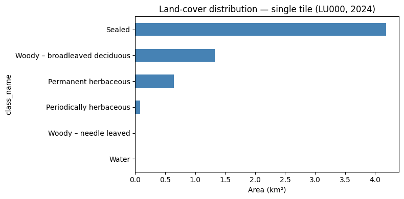
Goal: Create a horizontal bar chart showing the total area (km²) per land-cover class for the single tile.

Steps:

1. Set class_name as the index of stats_tile
2. Select the total_area_km2 column and sort values ascending
3. Plot as a horizontal bar chart with kind="barh"
4. Add axis label and title

import matplotlib.pyplot as plt

fig, ax = plt.subplots(figsize=(8, 4))

stats_tile.set_index("__")["__"].sort_values().plot(  # TODO: index column, value column
    kind="barh", ax=ax, color="steelblue"
)

ax.set_xlabel("__")  # TODO: axis label (str)
ax.set_title("__")   # TODO: chart title (str)
plt.tight_layout()
plt.show()

TipHint

• Index on "class_name", plot "total_area_km2".
• ax.set_xlabel("Area (km²)") and give a descriptive title.

TipSolution

import matplotlib.pyplot as plt

fig, ax = plt.subplots(figsize=(8, 4))

stats_tile.set_index("class_name")["total_area_km2"].sort_values().plot(
    kind="barh", ax=ax, color="steelblue"
)

ax.set_xlabel("Area (km²)")
ax.set_title("Land-cover distribution — single tile (LU000, 2024)")
plt.tight_layout()
plt.show()

2 Statistics on a NUTS3 / year pair

Scaling up to the full NUTS3 region gives a comprehensive picture of land-cover composition across all tiles, and allows direct comparison with the individual tile analysed above.

2.1 Load the predictions

nuts_id = "LU000"
year = 2024

response_nuts = requests.get(
    f"{api_url}/predict_nuts",
    params={"nuts_id": nuts_id, "year": year},
)

gdf_nuts = gpd.GeoDataFrame.from_features(
    json.loads(response_nuts.json()["predictions"])["features"],
    crs="EPSG:3035",
)

gdf_nuts["area_m2"]    = gdf_nuts.geometry.area
gdf_nuts["area_km2"]   = gdf_nuts["area_m2"] / 1e6
gdf_nuts["class_name"] = gdf_nuts["label"].map(class_names)

2.2 Compute area statistics per class

CautionExercise 4 — Compute land-cover statistics for the full NUTS3 region

Goal: Apply the same aggregation as Exercise 1, but on gdf_nuts. Then compare class shares between the single tile and the full region in a GT table.

Steps:

1. Repeat the .groupby().agg() pattern from Exercise 1 on gdf_nuts
2. Compute total_nuts_km2 and add share_pct
3. Display the stats table with GT
4. Build a side-by-side comparison of tile vs. NUTS3 shares and display with GT

stats_nuts = (
    gdf_nuts.groupby(["label", "class_name"])
    .agg(
        n_polygons           = ("geometry", "count"),
        total_area_km2       = ("area_km2", "sum"),
        mean_polygon_area_m2 = ("area_m2",  "mean"),
        max_polygon_area_m2  = ("area_m2",  "max"),
    )
    .reset_index()
    .sort_values("total_area_km2", ascending=False)
)

total_nuts_km2 = __  # TODO: sum of total_area_km2
stats_nuts["share_pct"] = (__ / total_nuts_km2 * 100).round(2)  # TODO: column

(
    GT(stats_nuts, rowname_col="class_name")
    .tab_header(title="Land-cover statistics — LU000 NUTS3 (2024)")
    .cols_label(
        label                = "Label",
        n_polygons           = "N polygons",
        total_area_km2       = "Total area (km²)",
        mean_polygon_area_m2 = "Mean area (m²)",
        max_polygon_area_m2  = "Max area (m²)",
        share_pct            = "Share (%)",
    )
    .fmt_number(columns=["total_area_km2"], decimals=2)
    .fmt_number(columns=["mean_polygon_area_m2", "max_polygon_area_m2"], decimals=0)
    .fmt_number(columns=["share_pct"], decimals=1)
    .data_color(columns=["share_pct"], palette=["white", "steelblue"])
)

tile_shares = stats_tile.set_index("class_name")["share_pct"].rename("__")  # TODO: column name
nuts_shares = stats_nuts.set_index("class_name")["share_pct"].rename("__")  # TODO: column name

comparison = pd.concat([__, __], axis=1).fillna(0).reset_index()  # TODO: tile_shares, nuts_shares

(
    GT(comparison, rowname_col="class_name")
    .tab_header(title="Land-cover share — tile vs. NUTS3 (2024)")
    .cols_label(**{"tile_share_pct": "Tile (%)", "nuts3_share_pct": "NUTS3 (%)"})
    .fmt_number(decimals=1)
    .data_color(palette=["white", "steelblue"])
)

TipHint

• Same pattern as Exercise 1 — just replace gdf_tile with gdf_nuts.
• Rename the share columns "tile_share_pct" and "nuts3_share_pct".
• Call .reset_index() on the comparison DataFrame before passing to GT().

TipSolution

stats_nuts = (
    gdf_nuts.groupby(["label", "class_name"])
    .agg(
        n_polygons           = ("geometry", "count"),
        total_area_km2       = ("area_km2", "sum"),
        mean_polygon_area_m2 = ("area_m2",  "mean"),
        max_polygon_area_m2  = ("area_m2",  "max"),
    )
    .reset_index()
    .sort_values("total_area_km2", ascending=False)
)

total_nuts_km2 = stats_nuts["total_area_km2"].sum()
stats_nuts["share_pct"] = (stats_nuts["total_area_km2"] / total_nuts_km2 * 100).round(2)

(
    GT(stats_nuts, rowname_col="class_name")
    .tab_header(title="Land-cover statistics — LU000 NUTS3 (2024)")
    .cols_label(
        label                = "Label",
        n_polygons           = "N polygons",
        total_area_km2       = "Total area (km²)",
        mean_polygon_area_m2 = "Mean area (m²)",
        max_polygon_area_m2  = "Max area (m²)",
        share_pct            = "Share (%)",
    )
    .fmt_number(columns=["total_area_km2"], decimals=2)
    .fmt_number(columns=["mean_polygon_area_m2", "max_polygon_area_m2"], decimals=0)
    .fmt_number(columns=["share_pct"], decimals=1)
    .data_color(columns=["share_pct"], palette=["white", "steelblue"])
)

tile_shares = stats_tile.set_index("class_name")["share_pct"].rename("tile_share_pct")
nuts_shares = stats_nuts.set_index("class_name")["share_pct"].rename("nuts3_share_pct")
comparison  = pd.concat([tile_shares, nuts_shares], axis=1).fillna(0).reset_index()

(
    GT(comparison, rowname_col="class_name")
    .tab_header(title="Land-cover share — tile vs. NUTS3 (2024)")
    .cols_label(**{"tile_share_pct": "Tile (%)", "nuts3_share_pct": "NUTS3 (%)"})
    .fmt_number(decimals=1)
    .data_color(palette=["white", "steelblue"])
)

Land-cover share — tile vs. NUTS3 (2024)
	Tile (%)	NUTS3 (%)
Sealed	67.0	10.8
Woody – broadleaved deciduous	21.2	31.6
Permanent herbaceous	10.3	34.0
Periodically herbaceous	1.4	15.7
Woody – needle leaved	0.1	7.2
Water	0.0	0.3
Low-growing woody plants	0.0	0.2
Non- and sparsely-vegetated	0.0	0.1

Land-cover statistics — LU000 NUTS3 (2024)
	Label	N polygons	Total area (km²)	Mean area (m²)	Max area (m²)	Share (%)
Permanent herbaceous	6	39170	746.80	19,065	3,940,500	34.0
Woody – broadleaved deciduous	3	35817	694.25	19,383	4,814,300	31.6
Periodically herbaceous	7	6850	344.51	50,293	1,894,600	15.7
Sealed	1	22456	238.00	10,598	5,558,100	10.8
Woody – needle leaved	2	12655	157.53	12,448	1,907,000	7.2
Water	10	929	5.94	6,398	849,900	0.3
Low-growing woody plants	5	678	4.60	6,778	1,179,700	0.2
Non- and sparsely-vegetated	9	253	2.14	8,445	461,000	0.1

Land-cover share — tile vs. NUTS3 (2024)
	Tile (%)	NUTS3 (%)
Sealed	67.0	10.8
Woody – broadleaved deciduous	21.2	31.6
Permanent herbaceous	10.3	34.0
Periodically herbaceous	1.4	15.7
Woody – needle leaved	0.1	7.2
Water	0.0	0.3
Low-growing woody plants	0.0	0.2
Non- and sparsely-vegetated	0.0	0.1

2.3 Visualise the NUTS3 distribution

CautionExercise 5 — Plot area and share for the NUTS3 region

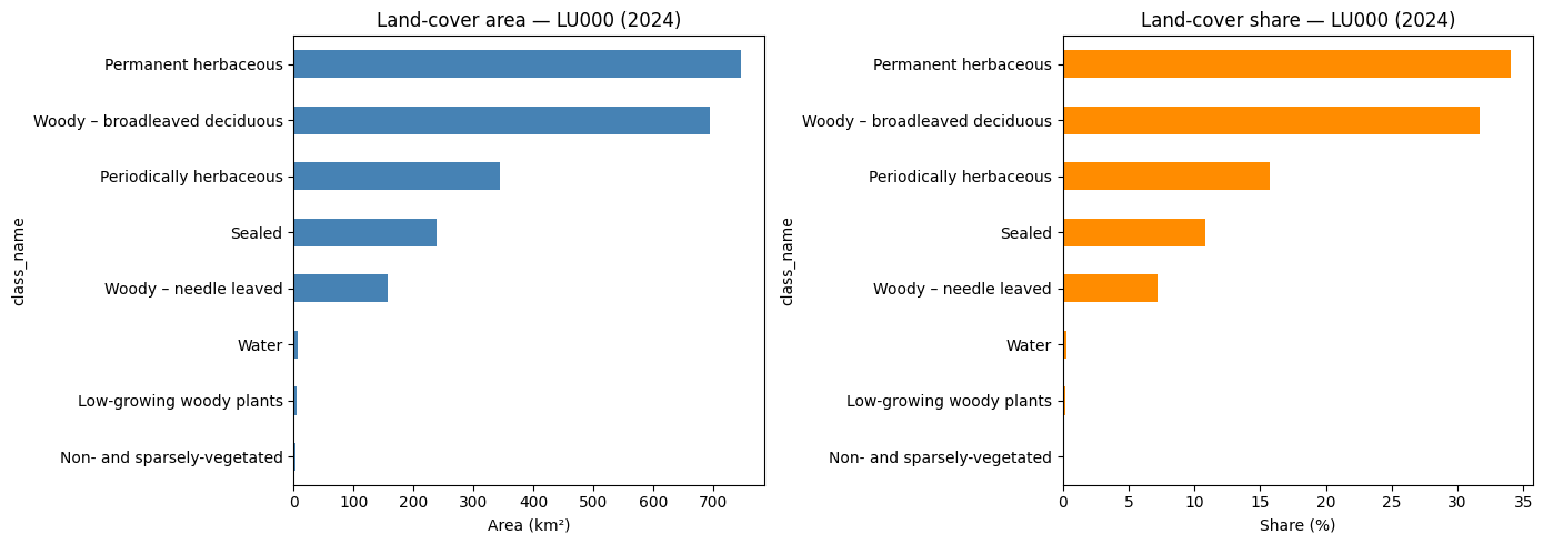
Goal: Create a two-panel figure showing (left) the total area in km² and (right) the share in % for each land-cover class across the full NUTS3 region.

Steps:

1. Create a figure with 2 side-by-side subplots
2. Plot total_area_km2 as a horizontal bar chart on the left panel
3. Plot share_pct as a horizontal bar chart on the right panel
4. Add labels and titles to both panels

fig, axes = plt.subplots(1, 2, figsize=(14, 5))

stats_nuts.set_index("class_name")["__"].sort_values().plot(  # TODO: column for left panel
    kind="barh", ax=axes[0], color="steelblue"
)
axes[0].set_xlabel("__")  # TODO: axis label
axes[0].set_title("__")   # TODO: title

stats_nuts.set_index("class_name")["__"].sort_values().plot(  # TODO: column for right panel
    kind="barh", ax=axes[1], color="darkorange"
)
axes[1].set_xlabel("__")  # TODO: axis label
axes[1].set_title("__")   # TODO: title

plt.tight_layout()
plt.show()

TipHint

• Left panel: "total_area_km2", label "Area (km²)".
• Right panel: "share_pct", label "Share (%)".

TipSolution

fig, axes = plt.subplots(1, 2, figsize=(14, 5))

stats_nuts.set_index("class_name")["total_area_km2"].sort_values().plot(
    kind="barh", ax=axes[0], color="steelblue"
)
axes[0].set_xlabel("Area (km²)")
axes[0].set_title("Land-cover area — LU000 (2024)")

stats_nuts.set_index("class_name")["share_pct"].sort_values().plot(
    kind="barh", ax=axes[1], color="darkorange"
)
axes[1].set_xlabel("Share (%)")
axes[1].set_title("Land-cover share — LU000 (2024)")

plt.tight_layout()
plt.show()

2.4 Interactive map — sealed surface density

Rather than displaying individual predicted polygons, this map aggregates sealed surfaces into a heatmap. Each sealed polygon contributes a point at its centroid, weighted by its area in km². Zones with many large sealed polygons (dense urban areas) appear in red, while isolated or small sealed patches appear in blue or yellow.

CautionExercise 6 — Build a heatmap of sealed surface density

Goal: Display the spatial density of sealed surfaces (label 1) across the NUTS3 region using a folium.plugins.HeatMap. Each point represents the centroid of a sealed polygon, weighted by its area.

Steps:

1. Reproject gdf_nuts to EPSG:4326 and compute the map centre
2. Filter sealed polygons (label 1) from the reprojected GeoDataFrame
3. Compute the centroid of each sealed polygon
4. Build heat_data as a list of [lat, lon, weight] where weight is area_km2
5. Create a folium.Map and add a HeatMap layer with a red gradient

import folium
from folium.plugins import HeatMap

gdf_nuts_wgs84 = gdf_nuts.to_crs("__")  # TODO: target CRS for Folium (str)
nuts_center    = gdf_nuts_wgs84.geometry.centroid.union_all().centroid

gdf_sealed = gdf_nuts_wgs84[gdf_nuts_wgs84["label"] == __].copy()  # TODO: sealed label (int)
gdf_sealed["centroid"] = gdf_sealed.geometry.centroid

heat_data = [
    [row.centroid.__, row.centroid.__, row.area_km2]  # TODO: lat/lon attributes
    for _, row in gdf_sealed.iterrows()
]

m = folium.Map(location=[nuts_center.y, nuts_center.x], zoom_start=__)  # TODO: zoom level

HeatMap(
    __,         # TODO: heat_data
    radius=__,  # TODO: radius in pixels (int), e.g. 15
    blur=__,    # TODO: blur in pixels (int), e.g. 20
    max_zoom=13,
    gradient={0.4: "blue", 0.6: "yellow", 0.8: "orange", 1.0: "red"},
).add_to(m)

m

TipHint

• Reproject with .to_crs("EPSG:4326").
• Filter with gdf_nuts_wgs84[gdf_nuts_wgs84["label"] == 1].
• geometry.centroid gives a Point; access its coordinates with .y (latitude) and .x (longitude).
• heat_data must be a list of [lat, lon, weight] — use area_km2 as the weight so larger sealed polygons contribute more to the heatmap.
• radius=15 and blur=20 are good starting values; increase radius to smooth the map at lower zoom levels.

TipSolution

import folium
from folium.plugins import HeatMap

gdf_nuts_wgs84 = gdf_nuts.to_crs("EPSG:4326")
nuts_center    = gdf_nuts_wgs84.geometry.centroid.union_all().centroid

gdf_sealed = gdf_nuts_wgs84[gdf_nuts_wgs84["label"] == 1].copy()
gdf_sealed["centroid"] = gdf_sealed.geometry.centroid

heat_data = [
    [row.centroid.y, row.centroid.x, row.area_km2]
    for _, row in gdf_sealed.iterrows()
]

m = folium.Map(location=[nuts_center.y, nuts_center.x], zoom_start=10)

HeatMap(
    heat_data,
    radius=15,
    blur=20,
    max_zoom=13,
    gradient={0.4: "blue", 0.6: "yellow", 0.8: "orange", 1.0: "red"},
).add_to(m)

m

Make this Notebook Trusted to load map: File -> Trust Notebook

Make this Notebook Trusted to load map: File -> Trust Notebook

3 Evolution — land-cover change between 2021 and 2024

Comparing predictions across two years reveals how land cover has evolved. This section fetches predictions for both 2021 and 2024 — first for a single tile, then for the full NUTS3 region — and quantifies the change in class shares (in percentage points). The change (pp) column is colour-coded: green for gains, red for losses.

3.1 Single tile — 2021 vs 2024

CautionExercise 6 — Compare land-cover on a single tile between 2021 and 2024

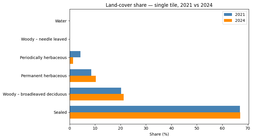
Goal: Fetch the 2021 prediction for the same tile, compute per-class statistics, compare shares with 2024, and display the result as a GT table with colour-coded change (pp) and a grouped bar chart.

Steps:

1. Call /predict_image with polygons=True for the 2021 tile path
2. Build gdf_tile_2021 with area and class name columns
3. Define compute_stats() and apply it to both years
4. Build tile_comparison with columns "2021 (%)", "2024 (%)", "change (pp)"
5. Display with GT — colour change (pp) red-white-green
6. Plot a grouped horizontal bar chart

image_filepath_2021 = (
    "projet-funathon/"
    "2026/project3/data/images/LU000/2021/"
    "__"  # TODO: same tile filename as 2024
)

response_2021 = requests.get(
    f"{api_url}/__",  # TODO: endpoint name
    params={"image": __, "polygons": __},
)

gdf_tile_2021 = gpd.GeoDataFrame.from_features(
    json.loads(response_2021.json())["features"],
    crs="EPSG:3035",
)

gdf_tile_2021["area_m2"]    = gdf_tile_2021.geometry.area
gdf_tile_2021["area_km2"]   = gdf_tile_2021["area_m2"] / 1e6
gdf_tile_2021["class_name"] = gdf_tile_2021["label"].map(class_names)


def compute_stats(gdf):
    stats = (
        gdf.groupby(["label", "class_name"])
        .agg(
            n_polygons           = ("geometry", "count"),
            total_area_km2       = ("area_km2", "sum"),
            mean_polygon_area_m2 = ("area_m2",  "mean"),
            max_polygon_area_m2  = ("area_m2",  "max"),
        )
        .reset_index()
        .sort_values("total_area_km2", ascending=False)
    )
    total = stats["total_area_km2"].sum()
    stats["share_pct"] = (stats["total_area_km2"] / total * 100).round(2)
    return stats, total


stats_tile_2021, _ = compute_stats(__)  # TODO: 2021 tile GeoDataFrame
stats_tile_2024, _ = compute_stats(__)  # TODO: 2024 tile GeoDataFrame

tile_2021 = stats_tile_2021.set_index("class_name")["share_pct"].rename("2021 (%)")
tile_2024 = stats_tile_2024.set_index("class_name")["share_pct"].rename("2024 (%)")

tile_comparison = pd.concat([tile_2021, tile_2024], axis=1).fillna(0)
tile_comparison["change (pp)"] = (tile_comparison["__"] - tile_comparison["__"]).round(2)

(
    GT(tile_comparison.reset_index(), rowname_col="class_name")
    .tab_header(title="Land-cover share — single tile, 2021 → 2024")
    .fmt_number(decimals=1)
    .data_color(
        columns=["change (pp)"],
        palette=["red", "white", "green"],
        domain=[-5, 5],
    )
    .data_color(columns=["2021 (%)", "2024 (%)"], palette=["white", "steelblue"])
)

fig, ax = plt.subplots(figsize=(9, 5))
x     = range(len(tile_comparison))
width = 0.35
ax.barh([i + width / 2 for i in x], tile_comparison["2021 (%)"], width, label="2021", color="steelblue")
ax.barh([i - width / 2 for i in x], tile_comparison["2024 (%)"], width, label="2024", color="darkorange")
ax.set_yticks(list(x))
ax.set_yticklabels(tile_comparison.index.tolist())
ax.set_xlabel("Share (%)")
ax.set_title("Land-cover share — single tile, 2021 vs 2024")
ax.legend()
plt.tight_layout()
plt.show()

TipHint

• The 2021 tile filename is identical to 2024 — only the year in the path changes.
• compute_stats(gdf) returns (stats_df, total_km2) — use _ to discard the total.
• change (pp) = "2024 (%)" - "2021 (%)" — positive means the class gained area share.
• data_color(columns=["change (pp)"], palette=["red", "white", "green"], domain=[-5, 5]) colours losses red and gains green automatically.

TipSolution

image_filepath_2021 = (
    "projet-funathon/"
    "2026/project3/data/images/LU000/2021/"
    "4042000_2951690_0_637.tif"
)

response_2021 = requests.get(
    f"{api_url}/predict_image",
    params={"image": image_filepath_2021, "polygons": True},
)

gdf_tile_2021 = gpd.GeoDataFrame.from_features(
    json.loads(response_2021.json())["features"],
    crs="EPSG:3035",
)

gdf_tile_2021["area_m2"]    = gdf_tile_2021.geometry.area
gdf_tile_2021["area_km2"]   = gdf_tile_2021["area_m2"] / 1e6
gdf_tile_2021["class_name"] = gdf_tile_2021["label"].map(class_names)


def compute_stats(gdf):
    stats = (
        gdf.groupby(["label", "class_name"])
        .agg(
            n_polygons           = ("geometry", "count"),
            total_area_km2       = ("area_km2", "sum"),
            mean_polygon_area_m2 = ("area_m2",  "mean"),
            max_polygon_area_m2  = ("area_m2",  "max"),
        )
        .reset_index()
        .sort_values("total_area_km2", ascending=False)
    )
    total = stats["total_area_km2"].sum()
    stats["share_pct"] = (stats["total_area_km2"] / total * 100).round(2)
    return stats, total


stats_tile_2021, _ = compute_stats(gdf_tile_2021)
stats_tile_2024, _ = compute_stats(gdf_tile)

tile_2021 = stats_tile_2021.set_index("class_name")["share_pct"].rename("2021 (%)")
tile_2024 = stats_tile_2024.set_index("class_name")["share_pct"].rename("2024 (%)")

tile_comparison = pd.concat([tile_2021, tile_2024], axis=1).fillna(0)
tile_comparison["change (pp)"] = (tile_comparison["2024 (%)"] - tile_comparison["2021 (%)"]).round(2)

(
    GT(tile_comparison.reset_index(), rowname_col="class_name")
    .tab_header(title="Land-cover share — single tile, 2021 → 2024")
    .fmt_number(decimals=1)
    .data_color(
        columns=["change (pp)"],
        palette=["red", "white", "green"],
        domain=[-5, 5],
    )
    .data_color(columns=["2021 (%)", "2024 (%)"], palette=["white", "steelblue"])
)

fig, ax = plt.subplots(figsize=(9, 5))
x     = range(len(tile_comparison))
width = 0.35
ax.barh([i + width / 2 for i in x], tile_comparison["2021 (%)"], width, label="2021", color="steelblue")
ax.barh([i - width / 2 for i in x], tile_comparison["2024 (%)"], width, label="2024", color="darkorange")
ax.set_yticks(list(x))
ax.set_yticklabels(tile_comparison.index.tolist())
ax.set_xlabel("Share (%)")
ax.set_title("Land-cover share — single tile, 2021 vs 2024")
ax.legend()
plt.tight_layout()
plt.show()

Land-cover share — single tile, 2021 → 2024
	2021 (%)	2024 (%)	change (pp)
Sealed	66.9	67.0	0.1
Woody – broadleaved deciduous	20.2	21.2	1.0
Permanent herbaceous	8.5	10.3	1.9
Periodically herbaceous	4.2	1.4	−2.9
Woody – needle leaved	0.1	0.1	−0.1
Water	0.0	0.0	0.0

3.2 NUTS3 region — 2021 vs 2024

CautionExercise 7 — Compare NUTS3 land-cover between 2021 and 2024

Goal: Scale up the temporal comparison to the full NUTS3 region. Fetch 2021 predictions from /predict_nuts, compute statistics, display a GT comparison table with colour-coded changes, an absolute area summary table, and a two-panel figure.

Steps:

1. Call /predict_nuts with nuts_id="LU000" and year=2021
2. Build gdf_nuts_2021 with area and class name columns
3. Apply compute_stats() to both years
4. Build nuts_comparison with "2021 (%)", "2024 (%)", "change (pp)"
5. Display with GT — colour change (pp) red-white-green
6. Build and display an absolute area summary table for the four key groups
7. Plot the two-panel figure

response_nuts_2021 = requests.get(
    f"{api_url}/__",  # TODO: endpoint name
    params={"nuts_id": "__", "year": __},  # TODO: LU000, 2021
)

gdf_nuts_2021 = gpd.GeoDataFrame.from_features(
    json.loads(response_nuts_2021.json()["__"])["features"],  # TODO: response key
    crs="EPSG:3035",
)

gdf_nuts_2021["area_m2"] = gdf_nuts_2021.geometry.area
gdf_nuts_2021["area_km2"] = gdf_nuts_2021["area_m2"] / 1e6
gdf_nuts_2021["class_name"] = gdf_nuts_2021["label"].map(class_names)

stats_nuts_2021, _ = compute_stats(__)  # TODO: 2021 NUTS3 GeoDataFrame
stats_nuts_2024, _ = compute_stats(__)  # TODO: 2024 NUTS3 GeoDataFrame

nuts_2021 = stats_nuts_2021.set_index("class_name")["share_pct"].rename("2021 (%)")
nuts_2024 = stats_nuts_2024.set_index("class_name")["share_pct"].rename("2024 (%)")

nuts_comparison = pd.concat([nuts_2021, nuts_2024], axis=1).fillna(0)
nuts_comparison["change (pp)"] = (nuts_comparison["__"] - nuts_comparison["__"]).round(2)

(
    GT(nuts_comparison.reset_index(), rowname_col="class_name")
    .tab_header(title="Land-cover share — LU000 NUTS3, 2021 → 2024")
    .fmt_number(decimals=1)
    .data_color(
        columns=["change (pp)"],
        palette=["red", "white", "green"],
        domain=[-5, 5],
    )
    .data_color(columns=["2021 (%)", "2024 (%)"], palette=["white", "steelblue"])
)

rows = []
for label, category in [
    (1, "Sealed"),
    ([2, 3, 4], "Forest"),
    ([6, 7], "Agricultural"),
    (10, "Water"),
]:
    labels_list = [label] if isinstance(label, int) else label
    km2_2021 = stats_nuts_2021.loc[stats_nuts_2021["label"].isin(labels_list), "total_area_km2"].sum()
    km2_2024 = stats_nuts_2024.loc[stats_nuts_2024["label"].isin(labels_list), "total_area_km2"].sum()
    rows.append({"Group": category, "2021 (km²)": round(km2_2021, 2),
                 "2024 (km²)": round(km2_2024, 2), "Δ (km²)": round(km2_2024 - km2_2021, 2)})

area_summary = pd.DataFrame(rows)

(
    GT(area_summary, rowname_col="Group")
    .tab_header(title="Absolute area change — LU000, 2021 → 2024")
    .fmt_number(decimals=2)
    .data_color(
        columns=["Δ (km²)"],
        palette=["red", "white", "green"],
        domain=[-10, 10],
    )
)

fig, axes = plt.subplots(1, 2, figsize=(14, 5))
x = range(len(nuts_comparison))
width = 0.35
labels = nuts_comparison.index.tolist()
axes[0].barh([i + width / 2 for i in x], nuts_comparison["2021 (%)"], width, label="2021", color="steelblue")
axes[0].barh([i - width / 2 for i in x], nuts_comparison["2024 (%)"], width, label="2024", color="darkorange")
axes[0].set_yticks(list(x))
axes[0].set_yticklabels(labels)
axes[0].set_xlabel("Share (%)")
axes[0].set_title("Land-cover share — LU000, 2021 vs 2024")
axes[0].legend()
colors = ["green" if v >= 0 else "red" for v in nuts_comparison["change (pp)"]]
axes[1].barh(labels, nuts_comparison["change (pp)"], color=colors)
axes[1].axvline(0, color="black", linewidth=0.8)
axes[1].set_xlabel("Change (percentage points)")
axes[1].set_title("Land-cover change 2021 → 2024 — LU000")
plt.tight_layout()
plt.show()

TipHint

• The response key for /predict_nuts is "predictions".
• compute_stats() is already defined in Exercise 6 — reuse it directly.
• change (pp) = "2024 (%)" - "2021 (%)".
• Build the absolute area summary as a pd.DataFrame with a loop over the four groups, then pass it to GT().
• For the change bar chart: colors = ["green" if v >= 0 else "red" for v in ...].

TipSolution

response_nuts_2021 = requests.get(
    f"{api_url}/predict_nuts",
    params={"nuts_id": "LU000", "year": 2021},
)

gdf_nuts_2021 = gpd.GeoDataFrame.from_features(
    json.loads(response_nuts_2021.json()["predictions"])["features"],
    crs="EPSG:3035",
)

gdf_nuts_2021["area_m2"] = gdf_nuts_2021.geometry.area
gdf_nuts_2021["area_km2"] = gdf_nuts_2021["area_m2"] / 1e6
gdf_nuts_2021["class_name"] = gdf_nuts_2021["label"].map(class_names)

stats_nuts_2021, _ = compute_stats(gdf_nuts_2021)
stats_nuts_2024, _ = compute_stats(gdf_nuts)

nuts_2021 = stats_nuts_2021.set_index("class_name")["share_pct"].rename("2021 (%)")
nuts_2024 = stats_nuts_2024.set_index("class_name")["share_pct"].rename("2024 (%)")

nuts_comparison = pd.concat([nuts_2021, nuts_2024], axis=1).fillna(0)
nuts_comparison["change (pp)"] = (nuts_comparison["2024 (%)"] - nuts_comparison["2021 (%)"]).round(2)

(
    GT(nuts_comparison.reset_index(), rowname_col="class_name")
    .tab_header(title="Land-cover share — LU000 NUTS3, 2021 → 2024")
    .fmt_number(decimals=1)
    .data_color(
        columns=["change (pp)"],
        palette=["red", "white", "green"],
        domain=[-5, 5],
    )
    .data_color(columns=["2021 (%)", "2024 (%)"], palette=["white", "steelblue"])
)

rows = []
for label, category in [
    (1,         "Sealed"),
    ([2, 3, 4], "Forest"),
    ([6, 7],    "Agricultural"),
    (10,        "Water"),
]:
    labels_list = [label] if isinstance(label, int) else label
    km2_2021 = stats_nuts_2021.loc[stats_nuts_2021["label"].isin(labels_list), "total_area_km2"].sum()
    km2_2024 = stats_nuts_2024.loc[stats_nuts_2024["label"].isin(labels_list), "total_area_km2"].sum()
    rows.append({"Group": category, "2021 (km²)": round(km2_2021, 2),
                 "2024 (km²)": round(km2_2024, 2), "Δ (km²)": round(km2_2024 - km2_2021, 2)})

area_summary = pd.DataFrame(rows)

(
    GT(area_summary, rowname_col="Group")
    .tab_header(title="Absolute area change — LU000, 2021 → 2024")
    .fmt_number(decimals=2)
    .data_color(
        columns=["Δ (km²)"],
        palette=["red", "white", "green"],
        domain=[-10, 10],
    )
)

fig, axes = plt.subplots(1, 2, figsize=(14, 5))
x      = range(len(nuts_comparison))
width  = 0.35
labels = nuts_comparison.index.tolist()
axes[0].barh([i + width / 2 for i in x], nuts_comparison["2021 (%)"], width, label="2021", color="steelblue")
axes[0].barh([i - width / 2 for i in x], nuts_comparison["2024 (%)"], width, label="2024", color="darkorange")
axes[0].set_yticks(list(x))
axes[0].set_yticklabels(labels)
axes[0].set_xlabel("Share (%)")
axes[0].set_title("Land-cover share — LU000, 2021 vs 2024")
axes[0].legend()
colors = ["green" if v >= 0 else "red" for v in nuts_comparison["change (pp)"]]
axes[1].barh(labels, nuts_comparison["change (pp)"], color=colors)
axes[1].axvline(0, color="black", linewidth=0.8)
axes[1].set_xlabel("Change (percentage points)")
axes[1].set_title("Land-cover change 2021 → 2024 — LU000")
plt.tight_layout()
plt.show()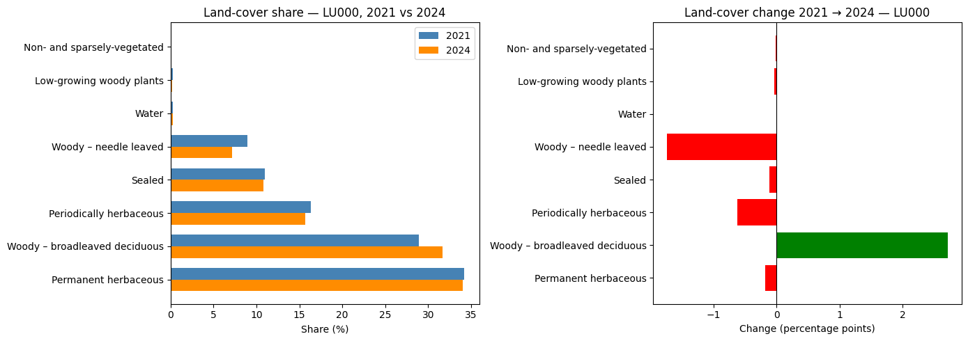

Land-cover share — LU000 NUTS3, 2021 → 2024
	2021 (%)	2024 (%)	change (pp)
Permanent herbaceous	34.2	34.0	−0.2
Woody – broadleaved deciduous	28.9	31.6	2.7
Periodically herbaceous	16.3	15.7	−0.6
Sealed	11.0	10.8	−0.1
Woody – needle leaved	8.9	7.2	−1.7
Water	0.3	0.3	0.0
Low-growing woody plants	0.2	0.2	−0.0
Non- and sparsely-vegetated	0.1	0.1	−0.0

Absolute area change — LU000, 2021 → 2024
	2021 (km²)	2024 (km²)	Δ (km²)
Sealed	240.59	238.00	−2.59
Forest	830.40	851.78	21.38
Agricultural	1,108.89	1,091.30	−17.59
Water	6.03	5.94	−0.08

3.3 Interactive map — forest gain and loss (2021 → 2024)

The statistics above show where forest cover has changed globally across the region. This map goes further by showing where exactly forest has appeared or disappeared between 2021 and 2024. Using a geometric overlay(), we isolate areas that genuinely gained or lost tree cover — the two layers are geometrically disjoint by construction, so there is no overlap.

CautionExercise 8 — Map forest gain and loss (2021 → 2024) with a heatmap

Goal: Display the spatial distribution of forest gain and loss across the NUTS3 region using two folium.plugins.HeatMap layers. Forest polygons (labels 2, 3, 4) are compared geometrically between 2021 and 2024 using .overlay(). Because gained and lost areas are computed as geometric differences, the two layers are spatially disjoint — no colour overlap.

Steps:

1. Filter forest polygons (labels 2, 3, 4) from both years in EPSG:3035
2. Dissolve each year into a single geometry with .dissolve()
3. Use .overlay(..., how="difference") twice: once for loss (in 2021, not in 2024) and once for gain (in 2024, not in 2021)
4. Recompute area_km2 after each overlay and filter out micro-polygons
5. Reproject to EPSG:4326, compute centroids, build heat_lost and heat_gained as [lat, lon, area_km2] lists
6. Create a folium.Map and add both HeatMap layers with distinct gradients, then add a LayerControl

import folium
from folium.plugins import HeatMap

FOREST_LABELS = [__, __, __]  # TODO: forest label integers

# Filter and dissolve forest polygons per year — stay in metric CRS
forest_2021 = (
    gdf_nuts_2021[gdf_nuts_2021["label"].isin(__)]  # TODO: forest labels
    .to_crs("__")                                    # TODO: metric CRS
    .dissolve()
    .reset_index(drop=True)
)
forest_2024 = (
    gdf_nuts[gdf_nuts["label"].isin(__)]             # TODO: forest labels
    .to_crs("__")                                    # TODO: metric CRS
    .dissolve()
    .reset_index(drop=True)
)

# Forest in 2021 but not 2024 = lost; forest in 2024 but not 2021 = gained
forest_lost   = forest_2021.overlay(__, how="__")  # TODO: reference layer, method
forest_gained = forest_2024.overlay(__, how="__")  # TODO: reference layer, method

# Recompute areas and drop slivers
for gdf in [forest_lost, forest_gained]:
    gdf["area_km2"] = gdf.geometry.area / 1e6

forest_lost   = forest_lost[forest_lost["area_km2"]     > __]  # TODO: threshold
forest_gained = forest_gained[forest_gained["area_km2"] > __]  # TODO: threshold

# Reproject and compute centroids
forest_lost_wgs84   = forest_lost.to_crs("__")    # TODO: CRS
forest_gained_wgs84 = forest_gained.to_crs("__")  # TODO: CRS

forest_lost_wgs84["centroid"]   = forest_lost_wgs84.geometry.centroid
forest_gained_wgs84["centroid"] = forest_gained_wgs84.geometry.centroid

heat_lost = [
    [row.centroid.__, row.centroid.__, row.area_km2]  # TODO: lat/lon attributes
    for _, row in forest_lost_wgs84.iterrows()
]
heat_gained = [
    [row.centroid.__, row.centroid.__, row.area_km2]  # TODO: lat/lon attributes
    for _, row in forest_gained_wgs84.iterrows()
]

center = forest_lost_wgs84.geometry.centroid.union_all().centroid
m = folium.Map(location=[center.y, center.x], zoom_start=__)  # TODO: zoom level

HeatMap(
    __,           # TODO: heat_lost
    radius=__, blur=__, max_zoom=13,
    gradient={0.4: "lightyellow", 0.65: "orange", 1.0: "red"},
    name="Forest loss 2021→2024",
).add_to(m)

HeatMap(
    __,           # TODO: heat_gained
    radius=__, blur=__, max_zoom=13,
    gradient={0.4: "lightgreen", 0.65: "forestgreen", 1.0: "darkgreen"},
    name="Forest gain 2021→2024",
).add_to(m)

folium.LayerControl().add_to(m)
m

TipHint

• Forest labels are 2, 3, 4 — use .isin([2, 3, 4]).
• .dissolve() merges all forest polygons of a year into one multipolygon, making the overlay faster and avoiding duplicate intersections.
• forest_2021.overlay(forest_2024, how="difference") → lost (in 2021, not 2024).
• forest_2024.overlay(forest_2021, how="difference") → gained (in 2024, not 2021).
• The two resulting layers are geometrically disjoint — no colour overlap.
• Use 1e-6 as the minimum area threshold to drop topological slivers.
• Reproject to "EPSG:4326" before computing centroids for Folium.
• radius=15 and blur=20 are good starting values.

TipSolution

import folium
from folium.plugins import HeatMap

FOREST_LABELS = [2, 3, 4]

forest_2021 = (
    gdf_nuts_2021[gdf_nuts_2021["label"].isin(FOREST_LABELS)]
    .to_crs("EPSG:3035")
    .dissolve()
    .reset_index(drop=True)
)
forest_2024 = (
    gdf_nuts[gdf_nuts["label"].isin(FOREST_LABELS)]
    .to_crs("EPSG:3035")
    .dissolve()
    .reset_index(drop=True)
)

forest_lost = forest_2021.overlay(forest_2024, how="difference")
forest_gained = forest_2024.overlay(forest_2021, how="difference")

forest_lost["area_km2"] = forest_lost.geometry.area / 1e6
forest_gained["area_km2"] = forest_gained.geometry.area / 1e6

forest_lost = forest_lost[forest_lost["area_km2"] > 1e-6]
forest_gained = forest_gained[forest_gained["area_km2"] > 1e-6]

forest_lost_wgs84 = forest_lost.to_crs("EPSG:4326")
forest_gained_wgs84 = forest_gained.to_crs("EPSG:4326")

forest_lost_wgs84["centroid"] = forest_lost_wgs84.geometry.centroid
forest_gained_wgs84["centroid"] = forest_gained_wgs84.geometry.centroid

heat_lost = [
    [row.centroid.y, row.centroid.x, row.area_km2]
    for _, row in forest_lost_wgs84.iterrows()
]
heat_gained = [
    [row.centroid.y, row.centroid.x, row.area_km2]
    for _, row in forest_gained_wgs84.iterrows()
]

center = forest_lost_wgs84.geometry.centroid.union_all().centroid
m = folium.Map(location=[center.y, center.x], zoom_start=11)

HeatMap(
    heat_lost,
    radius=15,
    blur=20,
    max_zoom=13,
    gradient={0.4: "lightyellow", 0.65: "orange", 1.0: "red"},
    name="Forest loss 2021→2024",
).add_to(m)

HeatMap(
    heat_gained,
    radius=15,
    blur=20,
    max_zoom=13,
    gradient={0.4: "lightgreen", 0.65: "forestgreen", 1.0: "darkgreen"},
    name="Forest gain 2021→2024",
).add_to(m)

folium.LayerControl().add_to(m)

<folium.map.LayerControl at 0x7f465a7f1400>

Make this Notebook Trusted to load map: File -> Trust Notebook

4 Be free to create new statistics and visualizations

The analyses above are just a starting point. Here are some ideas to go further:

• Spatial clustering: identify contiguous sealed zones above a certain area threshold to locate urban cores
• Per-tile breakdown: compute statistics tile by tile to map within-region heterogeneity
• Change detection map: build a Folium map where polygons are coloured by their change status (gained sealed, lost forest, stable, etc.)
• Ratio indicators: compute forest-to-sealed ratio or green infrastructure share per sub-region
• Time series: extend the comparison to all available years (2018–2024) and plot an area trend line per class