Inference

1 Load the Trained Model

This section covers how to load a trained segmentation model and apply it to a Sentinel-2 image to produce land-cover predictions.

1.1 From MLflow (optional)

If you completed the training step, you can load your registered model directly from the MLflow Model Registry instead of using the pre-trained checkpoint.

If you created a .env file at the root of your project (required when your MLflow service was launched after your VSCode service), it will be picked up automatically here.

Exercise 1 — Load a model from MLflow (optional)

Goal: Load a trained segmentation model from the MLflow model registry and retrieve its metadata (n_bands, tiles_size, augment_size, normalization parameters).

Steps:

Set model_name and model_version
Load the model from the registry with mlflow.pyfunc.load_model
Read the run parameters from mlflow.get_run()
Print the metadata to verify

import json
import os
import mlflow
import numpy as np
from dotenv import load_dotenv

load_dotenv()

model_name = __  # TODO: name of the model registered in MLflow (str)
model_version = __  # TODO: version of the model to load (str)
mlflow_tracking_uri = os.getenv("MLFLOW_TRACKING_URI")

mlflow.set_tracking_uri(mlflow_tracking_uri)
model = mlflow.pyfunc.load_model(model_uri=f"models:/{model_name}/{model_version}")

run = mlflow.get_run(model.metadata.run_id)

n_bands = __  # TODO: read "n_bands" from run.data.params and cast to int
tiles_size = __  # TODO: read "tiles_size" from run.data.params and cast to int
augment_size = __  # TODO: read "augment_size" from run.data.params and cast to int
module_name = __  # TODO: read "module_name" from run.data.params (str)

normalization_mean = json.loads(
    __  # TODO: read "normalization_mean" from run.data.params
)[:n_bands]

normalization_std = [
    float(v) for v in eval(
        __  # TODO: read "normalization_std" from run.data.params
    )
][:n_bands]

print(f"n_bands={n_bands}, tiles_size={tiles_size}, augment_size={augment_size}")
print(f"mean={normalization_mean}")
print(f"std={normalization_std}")

Hint

model_name and model_version are strings — check the MLflow UI to find the right values.
All parameters are stored in run.data.params as strings; cast them to int where needed (e.g. int(run.data.params["n_bands"])).
MLFLOW_TRACKING_URI is loaded from the .env file via load_dotenv() + os.getenv().
Print run.data.params to explore all available keys.

Solution

import json
import os
import mlflow
import numpy as np
from dotenv import load_dotenv

load_dotenv()

model_name = "segmentation-sentinel2-model"
model_version = "1"
mlflow_tracking_uri = os.getenv("MLFLOW_TRACKING_URI")

mlflow.set_tracking_uri(mlflow_tracking_uri)
model = mlflow.pyfunc.load_model(model_uri=f"models:/{model_name}/{model_version}")

run = mlflow.get_run(model.metadata.run_id)

n_bands = int(run.data.params["n_bands"])
tiles_size = int(run.data.params["tiles_size"])
augment_size = int(run.data.params["augment_size"])
module_name = run.data.params["module_name"]

normalization_mean = json.loads(
    run.data.params["normalization_mean"]
)[:n_bands]

normalization_std = [
    float(v) for v in eval(
        run.data.params["normalization_std"]
    )
][:n_bands]

1.2 Load a model from public S3

For this funathon, a pre-trained segmentation model is publicly available on MinIO — no MLflow credentials or account required. The model artifacts are stored at:

https://minio.lab.sspcloud.fr/projet-funathon/mlflow-artifacts/
1/88138b467a484c54b9935b66460413cd/artifacts/

Two artifacts are needed:

model/ — the full MLflow model directory (weights, code, environment)
a JSON file containing the training hyperparameters (n_bands, tiles_size, augment_size, normalization_mean, etc.)

The loading strategy is:

Use s3fs with anon=True to connect to MinIO without credentials
Download the model/ directory recursively to a local temporary folder
Load the model from that local folder with mlflow.pyfunc.load_model()
Fetch the file containing the parameters over HTTPS with requests and parse the hyperparameters

Exercise 1 bis — Load a pre-trained model from public S3

Goal: Download the pre-trained segmentation model from MinIO and load it locally, along with all the hyperparameters needed to run inference.

Steps:

Connect to MinIO anonymously with s3fs.S3FileSystem(anon=True)
Download the model/ directory recursively to a local temp folder
Load the model with mlflow.pyfunc.load_model()
Enter https://datalab.sspcloud.fr/file-explorer/projet-funathon/mlflow-artifacts/ 1/88138b467a484c54b9935b66460413cd/artifacts/ in your web search bar and look at the files in it. Find the file containing all theses parameters n_bands, tiles_size, augment_size, module_name, normalization_mean, normalization_std and load it.

import s3fs
import mlflow
import requests
import tempfile
import numpy as np
from pathlib import Path

fs = s3fs.S3FileSystem(
    anon=True,
    endpoint_url=__,  # TODO: MinIO endpoint URL (str)
)

s3_run_path = __ # TODO: S3 path to the run directory
s3_model_path   = s3_run_path + "model"
local_model_dir = Path(tempfile.mkdtemp()) / "model"

fs.get(__, __, recursive=__)  # TODO: download the model directory recursively

model = mlflow.pyfunc.load_model(__)  # TODO: local model directory path (str)

params_url = "https://minio.lab.sspcloud.fr/" + s3_run_path + __  # TODO: file containing the parameters

response = requests.get(params_url)
run_params = response.json()

n_bands            = __(run_params[__])  # TODO: cast to int
tiles_size         = __(run_params[__])  # TODO: cast to int
augment_size       = __(run_params[__])  # TODO: cast to int
module_name        = run_params[__]      # TODO: read as str
normalization_mean = run_params[__][:n_bands]  # TODO: key name
normalization_std  = run_params[__][:n_bands]  # TODO: key name

print(f"n_bands={n_bands}, tiles_size={tiles_size}, augment_size={augment_size}")
print(f"mean={normalization_mean}")
print(f"std={normalization_std}")

Hint

Pass anon=True to s3fs.S3FileSystem() for anonymous public access.
The MinIO endpoint URL is "https://minio.lab.sspcloud.fr".
The S3 path does not include s3:// — just the bucket and key: "projet-funathon/mlflow-artifacts/<id>/<run_id>/artifacts/model".
fs.get(src, dst, recursive=True) downloads the full directory tree.
mlflow.pyfunc.load_model() accepts a local directory path as a string.
The params.json URL follows the same structure as the model URL, replacing model with params.json.
All numeric parameters are stored as strings in JSON — cast with int().

Solution

import s3fs
import mlflow
import requests
import tempfile
import numpy as np
from pathlib import Path

fs = s3fs.S3FileSystem(
    anon=True,
    endpoint_url="https://minio.lab.sspcloud.fr",
)

s3_run_path = "projet-funathon/mlflow-artifacts/1/88138b467a484c54b9935b66460413cd/artifacts/"

s3_model_path = s3_run_path + "model"
local_model_dir = Path(tempfile.mkdtemp()) / "model"

fs.get(s3_model_path, str(local_model_dir), recursive=True)

model = mlflow.pyfunc.load_model(str(local_model_dir))

params_url = "https://minio.lab.sspcloud.fr/" + s3_run_path + "params.json"

response = requests.get(params_url)
run_params = response.json()

n_bands = int(run_params["n_bands"])
tiles_size = int(run_params["tiles_size"])
augment_size = int(run_params["augment_size"])
module_name = run_params["module_name"]
normalization_mean = run_params["normalization_mean"][:n_bands]
normalization_std = run_params["normalization_std"][:n_bands]

print(f"n_bands={n_bands}, tiles_size={tiles_size}, augment_size={augment_size}")
print(f"mean={normalization_mean}")
print(f"std={normalization_std}")

2 Apply the Model Locally

This section shows how to run inference locally — loading the image directly from MinIO over HTTPS, running the model, and post-processing the output.

2.1 Predict on a single Sentinel-2 image

The predict() function (in src/inference/prediction.py) handles the full pipeline — loading the image, preprocessing, tiling if needed, and assembling the result. It returns a tuple (satellite_img dict, predictions array) where predictions is a 2D integer array of shape (H, W) with class IDs from 1 to 10.

2.1.1 How `predict()` works

The SegFormer model was trained on fixed tiles_size × tiles_size patches. Real Sentinel-2 imagery is much larger, so predict() slices the input into model-sized pieces, predicts each piece, then stitches the per-pixel labels back into a single mask. The core branching looks like this:

si = get_satellite_image(image_path, n_bands)
if si["array"].shape[1] == tiles_size:        # already the right size
    return make_prediction(si, model, ...)
elif si["array"].shape[1] > tiles_size:       # larger → tile then mosaic
    tile_images = split_image(si, tiles_size)
    results = [make_prediction(t, model, ...) for t in tile_images]
    return make_mosaic(...)

Step by step:

Load — get_satellite_image() opens the GeoTIFF over HTTPS via GDAL’s /vsicurl/ virtual file system (no local download) and returns the pixel array together with its CRS, bounds and affine transform. Keeping the geospatial metadata is what lets us turn pixel predictions back into polygons with real-world coordinates later.
Tile — split_image() slices the array into tiles_size × tiles_size chunks. The full image must be an integer multiple of tiles_size, otherwise predict() raises an error — the SegFormer head only knows how to consume the exact patch size it saw at training time.
Preprocess — preprocess_image() wraps Albumentations to (a) normalise each band by subtracting normalization_mean and dividing by normalization_std (the channel-wise statistics computed on the training set), (b) optionally resize to augment_size if it differs from tiles_size, and (c) transpose (H, W, C) → (C, H, W) and add a batch dimension. Skipping normalisation is the most common cause of garbage predictions: the network’s weights only make sense for inputs in the statistical range it was trained on.
Forward pass — model.predict(normalized.numpy()) runs the wrapped PyTorch SegFormer (loaded via MLflow’s pyfunc interface) and returns raw logits of shape (1, n_classes, H′, W′). Logits are the model’s unbounded per-class scores before any softmax — large positive values mean “very likely this class”.
Match resolution — SegFormer’s segmentation head emits logits at a coarser resolution than the input (typically tiles_size / 4). The code calls torch.nn.functional.interpolate(..., mode="bilinear") to upsample back to tiles_size. Bilinear (not nearest-neighbour) interpolation is used here because logits are continuous scores; we’ll discretise to class IDs only in the next step.
Argmax — np.argmax(prediction, axis=0) collapses the class axis, picking the highest-scoring class at each pixel. The result is a 2D int32 array of class IDs.
Mosaic — when the image was tiled, make_mosaic() concatenates the tile labels row-by-row into the full mask and reuses the corner tiles’ CRS/bounds/transform so the assembled output is still georeferenced.

Note

This is why the metadata loaded from MLflow earlier — tiles_size, augment_size, normalization_mean, normalization_std, module_name — must travel with the model: inference has to reproduce the exact preprocessing used at training time. Mismatched values silently produce plausible-looking but incorrect predictions.

Exercise 2 — Run inference on a single Sentinel-2 image

Goal: Load a Sentinel-2 image from MinIO and run the segmentation model on it to produce a labelled mask.

Steps:

Build the full image URL by concatenating the base URL with image_target
Call predict() with the model and all metadata parameters
Print the mask shape and the set of predicted class IDs

from src.inference.prediction import predict

image_target = "LU000/2024/4022000_2979190_0_354.tif"

image_path = (
    "https://minio.lab.sspcloud.fr/projet-funathon/"
    "2026/project3/data/images/"
    + __  # TODO: relative path to the image (str), use image_target
)

satellite_img, predictions = predict(
    images=__,  # TODO: full image URL
    model=__,  # TODO: model loaded in Exercise 1
    tiles_size=__,  # TODO: tile size from model metadata
    augment_size=__,  # TODO: augmentation size from model metadata
    n_bands=__,  # TODO: number of bands
    normalization_mean=__,  # TODO: normalisation mean
    normalization_std=__,  # TODO: normalisation std
    module_name=__,  # TODO: module name
)

print(f"Mask shape : {predictions.shape}")
print(f"Classes found : {set(predictions.flatten().tolist())}")

Hint

Concatenate the base URL string with image_target to form image_path.
predict() returns a tuple (satellite_img dict, predictions array).
All metadata variables (tiles_size, augment_size, etc.) were retrieved in Exercise 1.

Solution

from src.inference.prediction import predict

image_target = "LU000/2024/4022000_2979190_0_354.tif"
image_path = (
    "https://minio.lab.sspcloud.fr/projet-funathon/"
    "2026/project3/data/images/" + image_target
)
satellite_img, predictions = predict(
    images=image_path,
    model=model,
    tiles_size=tiles_size,
    augment_size=augment_size,
    n_bands=n_bands,
    normalization_mean=normalization_mean,
    normalization_std=normalization_std,
    module_name=module_name,
)

print(f"Mask shape : {predictions.shape}")
print(f"Classes found : {set(predictions.flatten().tolist())}")

2.2 Display the prediction

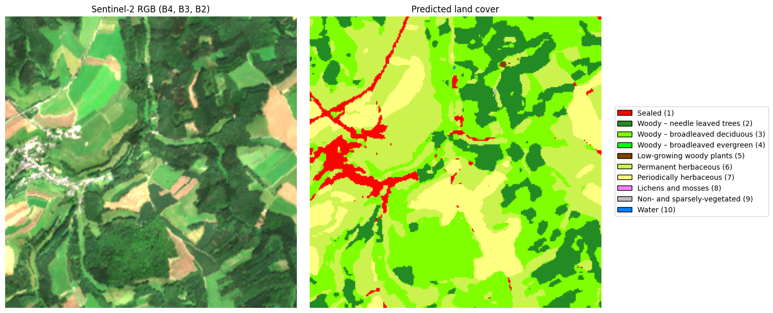
The 10 CLC+ Backbone land-cover classes are mapped to specific colours. A ListedColormap built from these colours ensures the mask and the legend are always consistent.

The RGB composite is built from bands 4, 3, 2 (Red, Green, Blue), which correspond to 0-based indices 3, 2, 1 in the array. A 98th-percentile normalisation avoids saturation from bright outliers.

Exercise 3 — Display the prediction

Goal: Build an RGB composite from the satellite image bands and display it side by side with the predicted land cover mask.

Steps:

Extract bands 4, 3, 2 (indices 3, 2, 1) and transpose to (H, W, 3), then normalise with the 98th percentile
Create a figure with 2 subplots (RGB / predicted mask)
Display rgb on axes[0] and predictions on axes[1] using cmap
Add a shared legend

import matplotlib.pyplot as plt
from matplotlib.colors import ListedColormap
from matplotlib.patches import Patch

# The 10 CLC+ Backbone classes — same set as defined in 1-acquisition.qmd § Exercise 10.
# Keep the order, IDs and hex colours in sync with that file (and with 5-statistics.qmd
# and map-nuts.qmd) so legends are consistent across the tutorial.
classes = [
    ("Sealed (1)",                        "#FF0100"),
    ("Woody – needle leaved trees (2)",   "#238B23"),
    ("Woody – broadleaved deciduous (3)", "#80FF00"),
    ("Woody – broadleaved evergreen (4)", "#00FF00"),
    ("Low-growing woody plants (5)",      "#804000"),
    ("Permanent herbaceous (6)",          "#CCF24E"),
    ("Periodically herbaceous (7)",       "#FEFF80"),
    ("Lichens and mosses (8)",            "#FF81FF"),
    ("Non- and sparsely-vegetated (9)",   "#BFBFBF"),
    ("Water (10)",                        "#0080FF"),
]

cmap = ListedColormap([color for _, color in classes])
label_to_color = {i + 1: color for i, (_, color) in enumerate(classes)}
legend_elements = [
    Patch(facecolor=color, edgecolor="black", label=label)
    for label, color in classes
]

# RGB composite — bands 4, 3, 2 → indices 3, 2, 1
satellite_img_array = satellite_img[__]  # TODO: array of the satellite image
rgb = np.transpose(
    satellite_img_array[[__, __, __]],  # TODO: band indices for R, G, B
    (1, 2, 0)
).astype(np.float32)
p98 = np.percentile(rgb, 98)
rgb = np.clip(rgb / p98, 0, 1)

fig, axes = plt.subplots(1, 2, figsize=(12, 6))

axes[0].imshow(__)                             # TODO: display the RGB composite
axes[0].set_title("Sentinel-2 RGB (B4, B3, B2)")
axes[0].axis("off")

axes[1].imshow(__, cmap=__, vmin=1, vmax=10)   # TODO: predictions array, colormap
axes[1].set_title("Predicted land cover")
axes[1].axis("off")

fig.legend(
    handles=legend_elements,
    loc="center left",
    bbox_to_anchor=(1.0, 0.5),
    frameon=True,
)
plt.tight_layout()
plt.show()

Hint

Sentinel-2 bands B4 / B3 / B2 are the Red / Green / Blue bands — feeding them to imshow produces a natural-colour (“true-colour”) image. Bands are named B1–B12 (1-indexed) but the array is 0-indexed, so B4=3, B3=2, B2=1.
satellite_img["array"] has shape (n_bands, H, W).
np.transpose(..., (1, 2, 0)) reshapes from (3, H, W) to (H, W, 3) — matplotlib expects channels-last.
Normalise: divide by np.percentile(rgb, 98) then np.clip(..., 0, 1). Using the 98th percentile (instead of the max) caps the few brightest outlier pixels and keeps the rest of the scene from looking washed out.
Use vmin=1, vmax=10 on imshow so the colormap aligns with the 10 CLC+ classes.

Solution

satellite_img_array = satellite_img["array"]
# Pick R/G/B (Sentinel-2 B4/B3/B2 → 0-indexed positions 3/2/1) and move
# channels last so matplotlib can render the natural-colour composite.
rgb = np.transpose(satellite_img_array[[3, 2, 1]], (1, 2, 0)).astype(np.float32)
# Cap brightness at the 98th percentile to avoid a few hot pixels washing out the image.
p98 = np.percentile(rgb, 98)
rgb = np.clip(rgb / p98, 0, 1)

fig, axes = plt.subplots(1, 2, figsize=(12, 6))

axes[0].imshow(rgb)
axes[0].set_title("Sentinel-2 RGB (B4, B3, B2)")
axes[0].axis("off")

axes[1].imshow(predictions, cmap=cmap, vmin=1, vmax=10)

axes[1].set_title("Predicted land cover")
axes[1].axis("off")

fig.legend(
    handles=legend_elements,
    loc="center left",
    bbox_to_anchor=(1.0, 0.5),
    frameon=True,
)

2.3 Convert predictions to polygons

create_geojson_from_mask() vectorises the class mask into a GeoDataFrame of polygons. Internally it writes the mask to a temporary GeoTIFF to preserve the georeference, then calls rasterio.features.shapes to extract contiguous regions of identical class. Each row in the output GeoDataFrame has a geometry (polygon) and a label (integer class ID from 1 to 10). Pixels with class value 0 (background / no-data) are automatically excluded.

Exercise 4 — Vectorise the mask and display the polygons

Goal: Convert the predicted mask into a GeoDataFrame of polygons, display the three outputs side by side (RGB / mask / polygons), and save the result.

Steps:

Call create_geojson_from_mask() with satellite_img and predictions
Create a 3-subplot figure: RGB on the left, mask in the centre, polygons on the right
Use gdf_pred.plot() with column="label" and the CLC+ colormap
Fix the axis limits of the polygon subplot with total_bounds

from src.inference.prediction import create_geojson_from_mask

gdf_pred = create_geojson_from_mask(__, __)  # TODO: satellite_img, predictions

print(f"{len(gdf_pred)} polygons extracted")
print(gdf_pred.head())

fig, axes = plt.subplots(1, 3, figsize=(20, 6))

axes[0].imshow(rgb)
axes[0].set_title("Sentinel-2 RGB (B4, B3, B2)")
axes[0].axis("off")

axes[1].imshow(predictions, cmap=cmap, vmin=1, vmax=10)
axes[1].set_title("Predicted land cover")
axes[1].axis("off")

gdf_pred.plot(
    column=__,  # TODO: column to use for colouring (str)
    cmap=__,    # TODO: colormap
    vmin=1, vmax=10,
    ax=axes[2],
    legend=False,
)
axes[2].set_title("Predicted polygons")
axes[2].set_aspect("equal")
xmin, ymin, xmax, ymax = gdf_pred.total_bounds
axes[2].set_xlim(xmin, xmax)
axes[2].set_ylim(ymin, ymax)
axes[2].axis("off")

fig.legend(handles=legend_elements, loc="center left", bbox_to_anchor=(1.0, 0.5), frameon=True)
plt.show()

Hint

create_geojson_from_mask(satellite_img, predictions) returns a GeoDataFrame with columns "geometry" and "label".
Use column="label" in gdf_pred.plot() to colour polygons by class.
After gdf_pred.plot(), geopandas resets the axis limits — use gdf_pred.total_bounds to restore them manually.

Solution

from src.inference.prediction import create_geojson_from_mask

gdf_pred = create_geojson_from_mask(satellite_img, predictions)

print(f"{len(gdf_pred)} polygons extracted")
print(gdf_pred.head())

fig, axes = plt.subplots(1, 3, figsize=(20, 6))

axes[0].imshow(rgb)
axes[0].set_title("Sentinel-2 RGB (B4, B3, B2)")
axes[0].axis("off")

axes[1].imshow(predictions, cmap=cmap, vmin=1, vmax=10)
axes[1].set_title("Predicted land cover")
axes[1].axis("off")

gdf_pred.plot(
    column="label",
    cmap=cmap,
    vmin=1, vmax=10,
    ax=axes[2],
    legend=False,
)
axes[2].set_title("Predicted polygons")
axes[2].set_aspect("equal")
xmin, ymin, xmax, ymax = gdf_pred.total_bounds
axes[2].set_xlim(xmin, xmax)
axes[2].set_ylim(ymin, ymax)
axes[2].axis("off")

fig.legend(handles=legend_elements, loc="center left", bbox_to_anchor=(1.0, 0.5), frameon=True)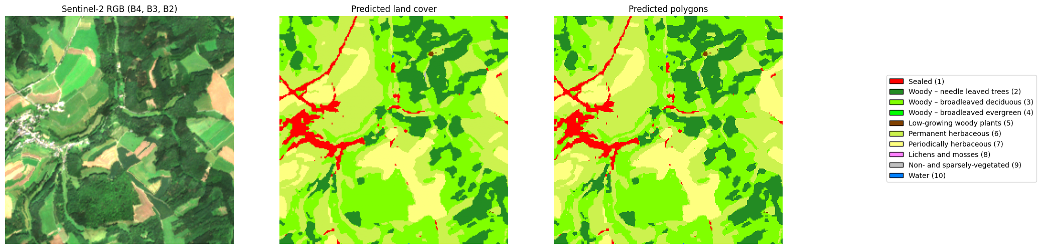

2.4 Display predictions on an interactive map

Folium renders interactive web maps directly in a Jupyter notebook. The satellite image is overlaid as a semi-transparent raster layer using ImageOverlay, while the predicted polygons are added as a GeoJson layer with per-class colouring.

Both layers must be in EPSG:4326 (WGS84, latitude/longitude) for Folium to place them correctly. transform_bounds() reprojects the raster bounding box, and gdf_pred.to_crs("EPSG:4326") reprojects the vector polygons.

Each layer is wrapped in a folium.FeatureGroup so that a LayerControl widget lets the user toggle them on and off independently directly on the map.

Exercise 5 — Display predictions on an interactive Folium map with layer control

Goal: Overlay the RGB image and the predicted polygons on an interactive Folium map as two independent toggleable layers.

Steps:

Reproject the image bounds to EPSG:4326 with transform_bounds()
Create a folium.Map centred on the tile
Create a FeatureGroup named "Sentinel-2 RGB" and add an ImageOverlay to it, then add the group to the map
Create a FeatureGroup named "Predicted polygons" and add a GeoJson layer coloured by label to it, then add the group to the map
Add a folium.LayerControl(collapsed=False) to display the toggle widget

import folium
from folium.raster_layers import ImageOverlay
from rasterio.warp import transform_bounds, reproject, Resampling, calculate_default_transform
from rasterio.crs import CRS

src_crs = si["crs"]
src_transform = si["transform"]
src_bounds = si["bounds"]
dst_crs = CRS.from_epsg(4326)

raw_bands = si["array"][[3, 2, 1]].astype(np.float32)
h, w = raw_bands.shape[1], raw_bands.shape[2]
dst_transform, dst_w, dst_h = calculate_default_transform(
    src_crs, dst_crs, w, h, *src_bounds
)
rgb_wgs84_bands = np.zeros((3, dst_h, dst_w), dtype=np.float32)
for i in range(3):
    reproject(
        source=raw_bands[i], destination=rgb_wgs84_bands[i],
        src_transform=src_transform, src_crs=src_crs,
        dst_transform=dst_transform, dst_crs=dst_crs,
        resampling=Resampling.bilinear,
    )
p98 = np.percentile(rgb_wgs84_bands[rgb_wgs84_bands > 0], 98)
rgb_wgs84 = np.clip(np.transpose(rgb_wgs84_bands, (1, 2, 0)) / p98, 0, 1)
alpha = (rgb_wgs84_bands.max(axis=0) > 0).astype(np.float32)
rgba_wgs84 = np.dstack([rgb_wgs84, alpha])

west, south, east, north = transform_bounds(src_crs, dst_crs, *src_bounds)
center_lat = (south + north) / 2
center_lon = (west + east) / 2

m = folium.Map(location=[center_lat, center_lon], zoom_start=14)

# Layer 1 — RGB image
fg_image = folium.FeatureGroup(name="__", show=__)  # TODO: layer name (str), show by default (bool)
ImageOverlay(
    image=__,                              # TODO: warped RGBA array (rgba_wgs84)
    bounds=[[south, west], [north, east]],
    opacity=0.7,
).add_to(__)  # TODO: add to fg_image
__.add_to(m)  # TODO: add fg_image to map

# Layer 2 — Predictions
fg_pred = folium.FeatureGroup(name="__", show=__)  # TODO: layer name (str), show by default (bool)
gdf_pred_wgs84 = gdf_pred.to_crs("__")  # TODO: target EPSG code for Folium (str)
folium.GeoJson(
    gdf_pred_wgs84,
    style_function=lambda feature: {
        "fillColor": __,  # TODO: use label_to_color to colour by label
        "color": "black",
        "weight": 0.5,
        "fillOpacity": 0.6,
    },
    tooltip=folium.GeoJsonTooltip(fields=["label"], aliases=["Class:"]),
).add_to(__)  # TODO: add to fg_pred
__.add_to(m)  # TODO: add fg_pred to map

# Layer control toggle widget
folium.LayerControl(collapsed=__).add_to(m)  # TODO: collapsed (bool)

m

Hint

transform_bounds(src_crs, "EPSG:4326", *bounds) returns (west, south, east, north) in decimal degrees.
Folium always expects coordinates in EPSG:4326.
Pass rgba_wgs84 (the EPSG:4326-warped RGBA array) to ImageOverlay. The alpha channel makes the triangular corners from the reprojection transparent rather than black.
feature["properties"]["label"] gives the integer class ID; use label_to_color.get(..., "#808080") for a safe fallback.
Each layer goes into a folium.FeatureGroup(name="...", show=True); call .add_to(fg) on the layer, then .add_to(m) on the group.
folium.LayerControl(collapsed=False) keeps the widget open by default.

Note

In Exercise 5, si refers to satellite_img loaded from local inference. In Exercise 8 (API section), si will be loaded via get_satellite_image().

Solution

import folium
from folium.raster_layers import ImageOverlay
from rasterio.warp import transform_bounds, reproject, Resampling, calculate_default_transform
from rasterio.crs import CRS

# Folium / Leaflet only render WGS84 (EPSG:4326, lat/lon). The Sentinel-2 tile
# lives in EPSG:3035 (metric projection used across Europe), so both the raster
# and the prediction polygons must be reprojected before they reach the map.
src_crs = satellite_img["crs"]
src_transform = satellite_img["transform"]
src_bounds = satellite_img["bounds"]
dst_crs = CRS.from_epsg(4326)

raw_bands = satellite_img_array[[3, 2, 1]].astype(np.float32)
h, w = raw_bands.shape[1], raw_bands.shape[2]
# calculate_default_transform picks an output grid in EPSG:4326 that covers the
# same area; reproject() then resamples each band onto that grid.
dst_transform, dst_w, dst_h = calculate_default_transform(
    src_crs, dst_crs, w, h, *src_bounds
)
rgb_wgs84_bands = np.zeros((3, dst_h, dst_w), dtype=np.float32)
for i in range(3):
    reproject(
        source=raw_bands[i], destination=rgb_wgs84_bands[i],
        src_transform=src_transform, src_crs=src_crs,
        dst_transform=dst_transform, dst_crs=dst_crs,
        resampling=Resampling.bilinear,  # bilinear for continuous reflectance values
    )
p98 = np.percentile(rgb_wgs84_bands[rgb_wgs84_bands > 0], 98)
rgb_wgs84 = np.clip(np.transpose(rgb_wgs84_bands, (1, 2, 0)) / p98, 0, 1)
# Reprojection from a tilted source produces empty triangular corners. Build an
# alpha channel from "where was there any data?" so those corners stay transparent.
alpha = (rgb_wgs84_bands.max(axis=0) > 0).astype(np.float32)
rgba_wgs84 = np.dstack([rgb_wgs84, alpha])

west, south, east, north = transform_bounds(src_crs, dst_crs, *src_bounds)
center_lat = (south + north) / 2
center_lon = (west + east) / 2

m = folium.Map(location=[center_lat, center_lon], zoom_start=14)

fg_image = folium.FeatureGroup(name="Sentinel-2 RGB", show=True)
ImageOverlay(
    image=rgba_wgs84,
    bounds=[[south, west], [north, east]],
    opacity=0.7,
).add_to(fg_image)
fg_image.add_to(m)

fg_pred = folium.FeatureGroup(name="Predicted polygons", show=True)
gdf_pred_wgs84 = gdf_pred.to_crs("EPSG:4326")  # vector polygons reprojected for Folium
folium.GeoJson(
    gdf_pred_wgs84,
    style_function=lambda feature: {
        "fillColor": label_to_color.get(feature["properties"]["label"], "#808080"),
        "color": "black",
        "weight": 0.5,
        "fillOpacity": 0.6,
    },
    tooltip=folium.GeoJsonTooltip(fields=["label"], aliases=["Class:"]),
).add_to(fg_pred)
fg_pred.add_to(m)

folium.LayerControl(collapsed=False).add_to(m)

m

Make this Notebook Trusted to load map: File -> Trust Notebook

3 Inference via API

Running inference locally works well for a single tile, but scaling to an entire NUTS3 region — which may contain dozens of tiles — requires more infrastructure. A REST API has been deployed for this purpose. The API’s interactive documentation is available at https://funathon-2026-project3-api.lab.sspcloud.fr/docs. It lists all available endpoints and lets you test them directly from your browser.

3.1 Architecture

The API is built with FastAPI and deployed on the SSP Cloud Kubernetes cluster. It wraps the same predict() / create_geojson_from_mask() pipeline used locally, but adds two important features:

S3 cache layer: predictions are stored in S3 as .npy files after the first inference call. Subsequent requests for the same image load the cached result instead of re-running the model, which drastically reduces latency for repeated or batched queries.
Batch processing: the /predict_nuts endpoint automatically discovers all .tif tiles for a given NUTS3/year pair in S3, runs (or loads from cache) predictions for each one, and merges the results into a single GeoJSON response.

3.2 Endpoints

The API exposes four endpoints:

Endpoint	Description
`GET /find_nuts`	Returns the NUTS3 identifier that contains a given GPS point
`GET /find_image`	Returns the filepath of the Sentinel-2 tile that contains a given GPS point
`GET /predict_image`	Runs inference on a single image; optionally returns vectorised polygons
`GET /predict_nuts`	Runs inference on all tiles for a NUTS3/year pair and returns merged polygons

3.2.1 `GET /find_nuts`

This endpoint identifies which NUTS3 region contains a given GPS point. It relies on the official Eurostat NUTS boundaries (NUTS_RG_01M_2021, level 3, EPSG:4326) loaded at startup. Internally, it performs a point-in-polygon spatial join to find the matching region.

This endpoint is used internally by /find_image when no nuts_id is provided by the caller: rather than scanning all available NUTS3 parquet indexes, the API first resolves the region from the coordinates, then queries only the relevant index.

Parameters:

Name	Type	Description
`gps_point`	`List[float, float]`	`[latitude, longitude]` in WGS84 (EPSG:4326)

Response: the NUTS3 identifier as a string (e.g. "LU000"), or an empty string if the point falls outside all known regions.

3.2.2 `GET /find_image`

This endpoint takes a GPS point ([latitude, longitude] in WGS84) and an optional NUTS3 identifier and year. It first resolves the NUTS3 region via /find_nuts if none is provided, then loads a pre-computed filename2bbox.parquet index from MinIO — a table that maps each tile filename to its bounding box in EPSG:3035 — and performs a spatial query to find which tile contains the point.

Parameters:

Name	Type	Description
`gps_point`	`List[float, float]`	`[latitude, longitude]` in WGS84 (EPSG:4326)
`year`	`int`	Year of the satellite images (2018–2024)
`nuts_id`	Optional `str`	NUTS3 region identifier, e.g. `"LU000"`. Resolved automatically if not provided.

Response: the S3 filepath of the tile containing the point (string), or an empty string if no tile is found.

3.2.3 `GET /predict_image`

This endpoint runs the full segmentation pipeline on a single Sentinel-2 tile identified by its S3 path. If a cached prediction already exists in S3, it is loaded directly without running the model again.

Parameters:

Name	Type	Description
`image`	`str`	S3 path to the `.tif` file
`polygons`	`bool`	If `True`, also vectorise the mask and return polygons (default: `False`)

Response: a GeoJSON string (FeatureCollection) containing the vectorised polygons when polygons=True, or an empty FeatureCollection otherwise.

3.2.4 `GET /predict_nuts`

This endpoint discovers all .tif tiles for a NUTS3/year pair in S3, runs (or loads from cache) predictions for each one, then concatenates the GeoDataFrames into a single response. This is the main entry point for region-level analysis.

Parameters:

Name	Type	Description
`nuts_id`	`str`	NUTS3 region identifier, e.g. `"LU000"`
`year`	`int`	Year of the satellite images (2018–2024)

Response: a GeoJSON string (FeatureCollection) containing all predicted polygons for the NUTS3 region, in EPSG:3035.

Note

The first call to /predict_nuts for a new NUTS3/year combination can take several minutes, as the model needs to run inference on every tile in the region. Subsequent calls are near-instant thanks to the S3 prediction cache.

3.3 Find the NUTS3 region from a GPS point

Exercise 6

Goal: Use the /find_nuts endpoint to identify the NUTS3 region that contains a GPS point of your choice.

Steps:

Choose any GPS point in Europe from Google Maps (right-click → copy coordinates)
Call GET /find_nuts with the correct parameters
Print the NUTS3 identifier returned by the API

import requests

api_url = "https://funathon-2026-project3-api.lab.sspcloud.fr"

gps_point = __    # TODO: [latitude, longitude] in WGS84 (List[float]), e.g. [49.63, 6.16]

response_nuts = requests.get(
    f"{api_url}/__",  # TODO: endpoint name (str)
    params={
        "gps_point": __,  # TODO: [latitude, longitude] defined above
    },
)
response_nuts.raise_for_status()

nuts_id = response_nuts.json()
print(f"NUTS3 region found: {nuts_id}")

Hint

The Eurostat offices in Luxembourg are at latitude=49.63, longitude=6.16.
The endpoint name is "find_nuts".
requests automatically repeats the parameter for each list value: [49.63, 6.16] → ?gps_point=49.63&gps_point=6.16.
The response is a plain string, e.g. "LU000".

Solution

import requests

api_url = "https://funathon-2026-project3-api.lab.sspcloud.fr"

gps_point = [49.63339525016761, 6.1689982433356025]  # [lat, lon]

response_nuts = requests.get(
    f"{api_url}/find_nuts",
    params={
        "gps_point": gps_point,
    },
)
response_nuts.raise_for_status()

nuts_id = response_nuts.json()
print(f"NUTS3 region found: {nuts_id}")

3.4 Find a satellite image from a GPS point

Exercise 7

Goal: Use the /find_image endpoint to find the Sentinel-2 tile that contains a GPS point in Luxembourg.

Steps:

Choose a GPS point in Luxembourg from Google Maps (e.g. the Eurostat offices)
Call GET /find_image with the correct parameters
Print the filename returned by the API

import json
import requests

api_url = "https://funathon-2026-project3-api.lab.sspcloud.fr"

gps_point = __    # TODO: [latitude, longitude] in WGS84 (List[float]), e.g. [49.63, 6.16] for Eurostat
year = __    # TODO: year of the satellite images (int, between 2018 and 2024)

response_find = requests.get(
    f"{api_url}/__",  # TODO: endpoint name (str), e.g. "find_image"
    params={
        "gps_point": __,  # TODO: [latitude, longitude] defined above
        "year": __,  # TODO: year defined above
    },
)
response_find.raise_for_status()

image_filename = response_find.json()
print(f"Image found: {image_filename}")

Hint

The Eurostat offices are at latitude=49.63, longitude=6.16.
The endpoint name is "find_image".
requests automatically repeats the parameter for each list value: [49.63, 6.16] → ?gps_point=49.63&gps_point=6.16.

Solution

import json
import requests

api_url = "https://funathon-2026-project3-api.lab.sspcloud.fr"

gps_point = [49.63339525016761, 6.1689982433356025]  # [lat, lon]
year = 2024

response_find = requests.get(
    f"{api_url}/find_image",
    params={
        "gps_point": gps_point,
        "year": year,
    },
)
response_find.raise_for_status()

image_filepath = response_find.json()
print(f"Image found: {image_filepath}")

3.5 Predict a single image via the API

Exercise 8

Goal: Call /predict_image with the filename found in Exercise 6 to retrieve the predicted polygons, then visualise them on a static plot.

Steps:

Call GET /predict_image with polygons=True
Parse the response as a GeoDataFrame
Load the RGB composite with get_satellite_image() and display 2 subplots

response_pred = requests.get(
    f"{api_url}/__",  # TODO: endpoint name (str), e.g. "predict_image"
    params={
        "image": __,  # TODO: S3 path built above
        "polygons": __,  # TODO: set to True to receive polygons
    },
)
response_pred.raise_for_status()

gdf_pred = gpd.GeoDataFrame.from_features(
    json.loads(response_pred.json())["features"],  # parse GeoJSON string → dict → features
    crs="EPSG:3035",
)

print(f"{len(gdf_pred)} polygons extracted")
print(gdf_pred.head())

import geopandas as gpd
from src.inference.prediction import get_satellite_image

N_BANDS = 14
minio_url = "https://minio.lab.sspcloud.fr/"

image_url = minio_url + __  # TODO: S3 image path built above (image_filepath)

si = get_satellite_image(__, n_bands=__)  # TODO: full HTTPS URL, number of bands

rgb = np.transpose(si["array"][[3, 2, 1]], (1, 2, 0)).astype(np.float32)
p98 = np.percentile(rgb, 98)
rgb = np.clip(rgb / p98, 0, 1)

fig, axes = plt.subplots(1, 2, figsize=(12, 6))

axes[0].imshow(rgb)
axes[0].set_title("Sentinel-2 RGB (B4, B3, B2)")
axes[0].axis("off")

gdf_pred.plot(column="label", cmap=cmap, vmin=1, vmax=10, ax=axes[1], legend=False)
axes[1].set_title("Predicted polygons")
axes[1].set_aspect("equal")
xmin, ymin, xmax, ymax = gdf_pred.total_bounds
axes[1].set_xlim(xmin, xmax)
axes[1].set_ylim(ymin, ymax)
axes[1].axis("off")

fig.legend(handles=legend_elements, loc="center left", bbox_to_anchor=(1.0, 0.5), frameon=True)
plt.show()

Hint

The endpoint name is "predict_image".
Set polygons=True to include GeoJSON polygons in the response.
response_pred.json() returns a GeoJSON string; json.loads() parses it into a dict before calling from_features().
get_satellite_image(url, n_bands=14) returns a dict with key "array" of shape (n_bands, H, W).
feature["properties"]["label"] gives the integer class ID; use label_to_color.get(..., "#808080") as a safe fallback.

Solution

import geopandas as gpd
from src.inference.prediction import get_satellite_image

response_pred = requests.get(
    f"{api_url}/predict_image",
    params={"image": image_filepath, "polygons": True},
)
response_pred.raise_for_status()

gdf_pred = gpd.GeoDataFrame.from_features(
    json.loads(response_pred.json())["features"],
    crs="EPSG:3035",
)

N_BANDS = 14
minio_url = "https://minio.lab.sspcloud.fr/"
image_url = minio_url + image_filepath
si = get_satellite_image(image_url, n_bands=N_BANDS)

rgb = np.transpose(si["array"][[3, 2, 1]], (1, 2, 0)).astype(np.float32)
p98 = np.percentile(rgb, 98)
rgb = np.clip(rgb / p98, 0, 1)

fig, axes = plt.subplots(1, 2, figsize=(12, 6))
axes[0].imshow(rgb)
axes[0].set_title("Sentinel-2 RGB (B4, B3, B2)")
axes[0].axis("off")
gdf_pred.plot(column="label", cmap=cmap, vmin=1, vmax=10, ax=axes[1], legend=False)
axes[1].set_title("Predicted polygons")
axes[1].set_aspect("equal")
xmin, ymin, xmax, ymax = gdf_pred.total_bounds
axes[1].set_xlim(xmin, xmax)
axes[1].set_ylim(ymin, ymax)
axes[1].axis("off")
fig.legend(handles=legend_elements, loc="center left", bbox_to_anchor=(1.0, 0.5), frameon=True)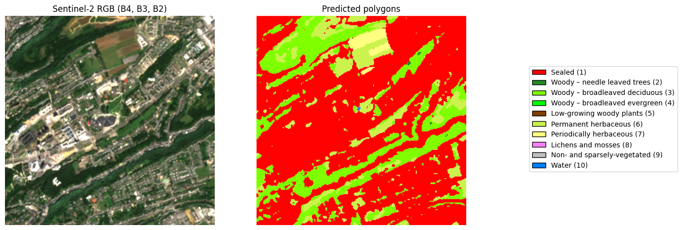

3.6 Predict an entire NUTS3 region

Exercise 9

Goal: Use /predict_nuts to retrieve predictions for all Sentinel-2 tiles covering Luxembourg (LU000) in 2024, visualise the result on a Folium map, and save it to a Parquet file.

Steps:

Call GET /predict_nuts with nuts_id="LU000" and year=2024
Parse the response as a GeoDataFrame
Print the number of polygons and the first rows
Display on a Folium map with per-class colouring
Save the Folium map to visualize it

nuts_id = "LU000"
year = 2024

response_nuts = requests.get(
    f"{api_url}/__",  # TODO: endpoint name (str), e.g. "predict_nuts"
    params={
        "nuts_id": "__",  # TODO: NUTS3 identifier (str), e.g. "LU000"
        "year":    __,    # TODO: year (int, between 2018 and 2024)
    },
)
response_nuts.raise_for_status()

gdf_nuts = gpd.GeoDataFrame.from_features(
    json.loads(response_nuts.json()["predictions"])["features"],  # parse GeoJSON string → dict → features
    crs="EPSG:3035",
)

print(f"{len(gdf_nuts)} polygons received")
print(gdf_nuts.head())

import folium
import numpy as np


# Reprojection
gdf_nuts_wgs84 = gdf_nuts.to_crs("EPSG:4326")
nuts_center = gdf_nuts_wgs84.geometry.centroid.union_all().centroid

m_nuts = folium.Map(location=[nuts_center.y, nuts_center.x], zoom_start=10)

# Layer 1 — Satellite imagery (Esri tile service, loaded on demand)
folium.TileLayer(
    tiles="https://server.arcgisonline.com/ArcGIS/rest/services/World_Imagery/MapServer/tile/{z}/{y}/{x}",
    attr="Esri",
    name="__",   # TODO: layer name (str), e.g. "Satellite imagery"
    show=__,     # TODO: visible by default (bool)
    overlay=True,
    control=True,
).add_to(m_nuts)

# Layer 2 — Predictions
fg_pred = folium.FeatureGroup(name="__", show=__)  # TODO: layer name (str), visible by default (bool)
folium.GeoJson(
    __,  # TODO: reprojected NUTS3 GeoDataFrame
    style_function=lambda feature: {
        "fillColor": __,  # TODO: use label_to_color to colour by label
        "color": "black",
        "weight": 0.3,
        "fillOpacity": 0.6,
    },
    tooltip=folium.GeoJsonTooltip(fields=["label"], aliases=["Class:"]),
).add_to(__)  # TODO: add to fg_pred
__.add_to(m_nuts)  # TODO: add fg_pred to map

folium.LayerControl(collapsed=__).add_to(m_nuts)  # TODO: collapsed (bool)

m_nuts.save("map_nuts.html")

Hint

Dissolve, then simplify, then reproject: gdf_nuts.dissolve(by="label").reset_index(), then gdf.geometry.simplify(500, preserve_topology=True) (500 m tolerance in EPSG:3035), then .to_crs("EPSG:4326"). The dissolve reduces features from thousands to 10; the simplification reduces vertex count ~50× so the rendered HTML stays a few MB instead of 150 MB.
Use folium.TileLayer(tiles=..., attr="Esri", name=..., show=True, overlay=True, control=True) and call .add_to(m_nuts) directly — no FeatureGroup needed for a tile layer.
Use FeatureGroup(name="Predicted polygons", show=True) for the predictions, then .add_to(fg_pred) on the GeoJson layer and .add_to(m_nuts) on the group.
label_to_color.get(feature["properties"]["label"], "#808080") colours polygons by class.
folium.LayerControl(collapsed=False) keeps the toggle widget open by default.

Solution

nuts_id = "LU000"
year = 2024

response_nuts = requests.get(
    f"{api_url}/predict_nuts",
    params={"nuts_id": nuts_id, "year": year},
)
response_nuts.raise_for_status()

gdf_nuts = gpd.GeoDataFrame.from_features(
    json.loads(response_nuts.json()["predictions"])["features"],
    crs="EPSG:3035",
)

print(f"{len(gdf_nuts)} polygons received")
print(gdf_nuts.head())

import folium
import numpy as np

gdf_nuts_wgs84 = gdf_nuts.to_crs("EPSG:4326")
nuts_center = gdf_nuts_wgs84.geometry.centroid.union_all().centroid

m_nuts = folium.Map(location=[nuts_center.y, nuts_center.x], zoom_start=10)

# Layer 1 — Satellite imagery (Esri tile service, loaded on demand)
folium.TileLayer(
    tiles="https://server.arcgisonline.com/ArcGIS/rest/services/World_Imagery/MapServer/tile/{z}/{y}/{x}",
    attr="Esri",
    name="Satellite imagery",
    show=True,
    overlay=True,
    control=True,
).add_to(m_nuts)

# Layer 2 — Predictions
fg_pred = folium.FeatureGroup(name="Predicted polygons", show=True)
folium.GeoJson(
    gdf_nuts_wgs84,
    style_function=lambda feature: {
        "fillColor": label_to_color.get(feature["properties"]["label"], "#808080"),
        "color": "black",
        "weight": 0.3,
        "fillOpacity": 0.6,
    },
    tooltip=folium.GeoJsonTooltip(fields=["label"], aliases=["Class:"]),
).add_to(fg_pred)
fg_pred.add_to(m_nuts)

folium.LayerControl(collapsed=False).add_to(m_nuts)

m_nuts.save("map_nuts.html")

1 Load the Trained Model

1.1 From MLflow (optional)

1.2 Load a model from public S3

2 Apply the Model Locally

2.1 Predict on a single Sentinel-2 image

2.1.1 How predict() works

2.2 Display the prediction

2.3 Convert predictions to polygons

2.4 Display predictions on an interactive map

3 Inference via API

3.1 Architecture

3.2 Endpoints

3.2.1 GET /find_nuts

3.2.2 GET /find_image

3.2.3 GET /predict_image

3.2.4 GET /predict_nuts

3.3 Find the NUTS3 region from a GPS point

3.4 Find a satellite image from a GPS point

3.5 Predict a single image via the API

3.6 Predict an entire NUTS3 region

2.1.1 How `predict()` works

3.2.1 `GET /find_nuts`

3.2.2 `GET /find_image`

3.2.3 `GET /predict_image`

3.2.4 `GET /predict_nuts`